Sparse Autoencoders in Deep Learning
Last Updated : 08 Apr, 2025
Sparse autoencoders are a specific form of autoencoder that's been trained for feature learning and dimensionality reduction. As opposed to regular autoencoders, which are trained to reconstruct the input data in the output, sparse autoencoders add a sparsity penalty that encourages the hidden layer to only use a limited number of neurons at any given time. The sparsity penalty causes the model to concentrate on the extraction of the most relevant features from the input data.
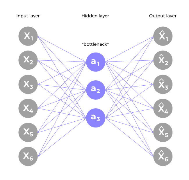 A simple single-layer sparse auto encoder with equal numbers of inputs (x), outputs (xhat) and hidden nodes (a).
 In a typical autoencoder, the network learns to encode and decode data without restrictions on the hidden layer’s activations. But sparse autoencoders go one step ahead by introducing a regularization term to avoid overfitting and forcing the learning of compact, interpretable features. This ensures that the network is not merely copying the input data but rather learns a compressed, meaningful representation of the data.
Objective Function of a Sparse Autoencoder
L = ||X - \hat{X}||^2 + \lambda \cdot \text{Penalty}(s)
- X: Input data.
- \hat{X}: Reconstructed output.
- \lambda: Regularization parameter.
- Penalty(s): A function that penalizes deviations from sparsity, often implemented using KL-divergence.
Techniques for Enforcing Sparsity
There are several methods to enforce the sparsity constraint:
- L1 Regularization: Introduces a penalty proportional to the absolute weight values, encouraging the model to utilize fewer features.
- KL Divergence: Estimates how much the average activation of hidden neurons deviates from the target sparsity level, such that a subset of neurons is activated at any time.
Training Sparse Autoencoders
Training a sparse autoencoder typically involves:
- Initialization: Weights are initialized randomly or using pre-trained networks.
- Forward Pass: The input is fed through the encoder to obtain the latent representation, followed by the decoder to reconstruct the output.
- Loss Calculation: The loss function is computed, incorporating both the reconstruction error and the sparsity penalty.
- Backpropagation: The gradients are calculated and used to update the weights.
Preventing the Autoencoder from Overfitting
Sparse autoencoders address an important issue in normal autoencoders: overfitting. In a normal autoencoder with an increased hidden layer, the network can simply "cheat" and replicate the input data to the output without deriving useful features. Sparse autoencoders address this by restricting how many of the hidden layer neurons are active at any given time, thus nudging the network to learn only the most critical features.
Implementation of a Sparse Autoencoder for MNIST Dataset
This is an implementation that shows how to construct a sparse autoencoder with TensorFlow and Keras in order to learn useful representations of the MNIST dataset. The model induces sparsity in the hidden layer activations, making it helpful for applications such as feature extraction.
Step 1: Import Libraries
We start by importing the libraries required for handling the data, constructing the model, and visualization.
Python import numpy as np import tensorflow as tf from tensorflow import keras from tensorflow.keras import layers import matplotlib.pyplot as plt
Step 2: Load and Preprocess the MNIST Dataset
We then load the MNIST dataset, which is a set of handwritten digits. We preprocess the data as well by reshaping and normalizing the pixel values.
- Reshaping: We convert the 28x28 images into a flat vector of size 784.
- Normalization: Pixel values are normalized to the range [0, 1].
Python (x_train, _), (x_test, _) = keras.datasets.mnist.load_data() x_train = x_train.reshape((x_train.shape[0], -1)).astype('float32') / 255.0 x_test = x_test.reshape((x_test.shape[0], -1)).astype('float32') / 255.0 Step 3: Define Model Parameters
We define the model parameters, including the input dimension, hidden layer size, sparsity level, and the sparsity regularization weight.
Python input_dim = 784 hidden_dim = 64 sparsity_level = 0.05 lambda_sparse = 0.1
Step 4: Build the Autoencoder Model
We construct the autoencoder model using Keras. The encoder reduces the dimension of the input data to lower dimensions, whereas the decoder attempts to recreate the original input based on this lower-dimensional representation.
Python inputs = layers.Input(shape=(input_dim,)) encoded = layers.Dense(hidden_dim, activation='relu')(inputs) decoded = layers.Dense(input_dim, activation='sigmoid')(encoded) autoencoder = keras.Model(inputs, decoded) encoder = keras.Model(inputs, encoded)
Step 5: Define the Sparse Loss Function
We create a custom loss function that includes both the mean squared error (MSE) and a sparsity penalty using KL divergence. This encourages the model to learn a sparse representation.
Python def sparse_loss(y_true, y_pred): mse_loss = tf.reduce_mean(keras.losses.MeanSquaredError()(y_true, y_pred)) hidden_layer_output = encoder(y_true) mean_activation = tf.reduce_mean(hidden_layer_output, axis=0) kl_divergence = tf.reduce_sum(sparsity_level * tf.math.log(sparsity_level / (mean_activation + 1e-10)) + (1 - sparsity_level) * tf.math.log((1 - sparsity_level) / (1 - mean_activation + 1e-10))) return mse_loss + lambda_sparse * kl_divergence
Step 6: Compile the Model
We compile the model with the Adam optimizer and the custom sparse loss function.
Python autoencoder.compile(optimizer='adam', loss=sparse_loss)
Step 7: Train the Autoencoder
The model is trained on the training data for a specified number of epochs. We shuffle the data to ensure better training.
Python history = autoencoder.fit(x_train, x_train, epochs=50, batch_size=256, shuffle=True)
Output:
Epoch 1/50
235/235 ━━━━━━━━━━━━━━━━━━━━ 4s 8ms/step - loss: 0.2632
. . .
Epoch 50/50
235/235 ━━━━━━━━━━━━━━━━━━━━ 2s 5ms/step - loss: 0.0281
Step 8: Reconstruct the Inputs
After training, we use the autoencoder to reconstruct the test data and visualize the results.
Python reconstructed = autoencoder.predict(x_test)
Step 9: Visualize Original vs. Reconstructed Images
We visualize the original images alongside their reconstructed counterparts to assess the model's performance.
Python n = 10 plt.figure(figsize=(20, 4)) for i in range(n): # Original images ax = plt.subplot(2, n, i + 1) plt.imshow(x_test[i].reshape(28, 28), cmap='gray') plt.title("Original") plt.axis('off') # Reconstructed images ax = plt.subplot(2, n, i + 1 + n) plt.imshow(reconstructed[i].reshape(28, 28), cmap='gray') plt.title("Reconstructed") plt.axis('off') plt.show() Output:
 Reconstructed Images
Step 10: Analyze Encoded Representations
We obtain the encoded representations and visualize them to understand the features learned by the autoencoder.
Python encoded_outputs = encoder.predict(x_train) # Visualize encoded features plt.figure(figsize=(10, 8)) plt.scatter(encoded_outputs[:, 0], encoded_outputs[:, 1]) # Assuming hidden_dim is 2 for visualization plt.title("Encoded Representations") plt.xlabel("Encoded Dimension 1") plt.ylabel("Encoded Dimension 2") plt.show() Output
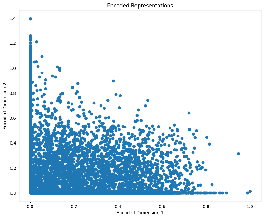 Encoded Representations
Step 11: Analyze Mean Activation of Hidden Units
Finally, we analyze the mean activation of the hidden units to understand how sparsity is achieved in the model.
Python mean_activation = np.mean(encoded_outputs, axis=0) plt.bar(range(len(mean_activation)), mean_activation) plt.title("Mean Activation of Hidden Units") plt.xlabel("Hidden Units") plt.ylabel("Mean Activation") plt.show() Output
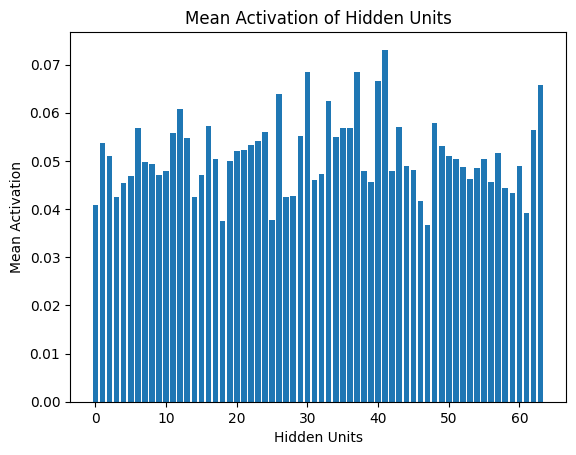 Mean Activation
Applications of Sparse Autoencoders
Sparse autoencoders have a wide range of applications in various fields:
- Feature Learning: They can be employed to learn a sparse representation of high-dimensional data, which can subsequently be employed for classification or regression purposes.
- Image Denoising: Sparse autoencoders can be employed to denoise images by learning to capture salient features and disregard unnecessary noise.
- Anomaly Detection: By training on normal data, sparse autoencoders can identify outliers based on reconstruction error.
- Data Compression: They can effectively compress data by reducing its dimensionality while retaining important features.
Advantages of Sparse Autoencoders
- Efficiency: They can learn efficient representations with fewer active neurons, leading to reduced computational costs.
- Interpretability: The sparsity constraint usually tends to create more interpretable features, which in turn can assist in interpreting the underlying structure of the data.
- Robustness: Sparse autoencoders have the potential to be more resistant to noise and overfitting because of the regularization effect they provide.