Gradient descent is an optimization algorithm used to find the values of parameters (coefficients) of a function (f) that minimizes a cost function. In other words, gradient descent is an iterative algorithm that helps to find the optimal solution to a given problem.
In this blog, we will discuss gradient descent optimization in TensorFlow, a popular deep-learning framework. TensorFlow provides several optimizers that implement different variations of gradient descent, such as stochastic gradient descent and mini-batch gradient descent.
Before diving into the details of gradient descent in TensorFlow, let's first understand the basics of gradient descent and how it works.
What is Gradient Descent?
Gradient descent is an iterative optimization algorithm that is used to minimize a function by iteratively moving in the direction of the steepest descent as defined by the negative of the gradient. In other words, the gradient descent algorithm takes small steps in the direction opposite to the gradient of the function at the current point, with the goal of reaching a global minimum.
The gradient of a function tells us the direction in which the function is increasing or decreasing the most. For example, if the gradient of a function is positive at a certain point, it means that the function is increasing at that point, and if the gradient is negative, it means that the function is decreasing at that point.
The gradient descent algorithm starts with an initial guess for the parameters of the function and then iteratively improves these guesses by taking small steps in the direction opposite to the gradient of the function at the current point. This process continues until the algorithm reaches a local or global minimum, where the gradient is zero (i.e., the function is not increasing or decreasing).
How does Gradient Descent work?
The gradient descent algorithm is an iterative algorithm that updates the parameters of a function by taking steps in the opposite direction of the gradient of the function. The gradient of a function tells us the direction in which the function is increasing or decreasing the most. The gradient descent algorithm uses the gradient to update the parameters in the direction that reduces the value of the cost function.
The gradient descent algorithm works in the following way:
- Initialize the parameters of the function with some random values.
- Calculate the gradient of the cost function with respect to the parameters.
- Update the parameters by taking a small step in the opposite direction of the gradient.
- Repeat steps 2 and 3 until the algorithm reaches a local or global minimum, where the gradient is zero.
- Here is a simple example to illustrate the gradient descent algorithm in action. Let's say we have a function f(x) = x2, and we want to find the value of x that minimizes the function. We can use the gradient descent algorithm to find this value.
First, we initialize the value of x with some random value, say x = 3. Next, we calculate the gradient of the function with respect to x, which is 2x. In this case, the gradient is 6 (2 * 3). Since the gradient is positive, it means that the function is increasing at x = 3, and we need to take a step in the opposite direction to reduce the value of the function.
We update the value of x by subtracting a small step size (called the learning rate) from the current value of x. For example, if the learning rate is 0.1, we can update the value of x as follows:
x = x - 0.1 * gradient
  = 3 - 0.1 * 6
  = 2.4
We repeat this process until the algorithm reaches a local or global minimum. To implement gradient descent in TensorFlow, we first need to define the cost function that we want to minimize. In this example, we will use a simple linear regression model to illustrate how gradient descent works.
Linear regression is a popular machine learning algorithm that is used to model the relationship between a dependent variable (y) and one or more independent variables (x). In a linear regression model, we try to find the best-fit line that describes the relationship between the dependent and independent variables. To create a linear regression model in TensorFlow, we first need to define the placeholders for the input and output data. A placeholder is a TensorFlow variable that we can use to feed data into our model.
Here is the code to define the placeholders for the input and output data:
Python # Import tensorflow 2 as tensorflow 1 import tensorflow.compat.v1 as tf tf.disable_v2_behavior() # Define the placeholders for # the input and output data x = tf.placeholder(tf.float32) y = tf.placeholder(tf.float32) # Define the placeholders for # the input and output data x = tf.placeholder(tf.float32) y = tf.placeholder(tf.float32)
Next, we need to define the variables that represent the parameters of our linear regression model. In this example, we will use a single variable (w) to represent the slope of the best-fit line. We initialize the value of w with a random value, say 0.5.
Here is the code to define the variable for the model parameters:
Python # Define the model parameters w = tf.Variable(0.5, name="weights")
Once we have defined the placeholders and the model parameters, we can define the linear regression model by using the TensorFlow tf.add() and tf.multiply() functions. The tf.add() function is used to add the bias term to the model, and the tf.multiply() function is used to multiply the input data (x) and the model parameters (w).
Here is the code to define the linear regression model:
Python # Define the linear regression model model = tf.add(tf.multiply(x, w), 0.5)
Once we have defined the linear regression model, we need to define the cost function that we want to minimize. In this example, we will use the mean squared error (MSE) as the cost function. The MSE is a popular metric that is used to evaluate the performance of a linear regression model. It measures the average squared difference between the predicted values and the actual values.
To define the cost function, we first need to calculate the difference between the predicted values and the actual values using the TensorFlow tf.square() function. The tf.square() function squares each element in the input tensor and returns the squared values.
Here is the code to define the cost function using the MSE:
Python # Define the cost function (MSE) cost = tf.reduce_mean(tf.square(model - y))
Once we have defined the cost function, we can use the TensorFlow tf.train.GradientDescentOptimizer() function to create an optimizer that uses the gradient descent algorithm to minimize the cost function. The tf.train.GradientDescentOptimizer() function takes the learning rate as an input parameter. The learning rate is a hyperparameter that determines the size of the steps that the algorithm takes to reach the minimum of the cost function.
Here is the code to create the gradient descent optimizer:
Python # Create the gradient descent optimizer optimizer = tf.train.GradientDescentOptimizer(learning_rate=0.01)
Once we have defined the optimizer, we can use the minimize() method of the optimizer to minimize the cost function. The minimize() method takes the cost function as an input parameter and returns an operation that, when executed, performs one step of gradient descent on the cost function.
Here is the code to minimize the cost function using the gradient descent optimizer:
Python # Minimize the cost function train = optimizer.minimize(cost)
Once we have defined the gradient descent optimizer and the train operation, we can use the TensorFlow Session class to train our model. The Session class provides a way to execute TensorFlow operations. To train the model, we need to initialize the variables that we have defined earlier (i.e., the model parameters and the optimizer) and then run the train operation in a loop for a specified number of iterations.
Here is the code to train the linear regression model using the gradient descent optimizer:
Python # Define the toy dataset x_train = [1, 2, 3, 4] y_train = [2, 4, 6, 8] # Create a TensorFlow session with tf.Session() as sess: # Initialize the variables sess.run(tf.global_variables_initializer()) # Training loop for i in range(1000): sess.run(train, feed_dict={x: x_train, y: y_train}) # Evaluate the model w_val = sess.run(w) # Mean Squared Error (MSE) between # the predicted and true output values print(w_val) In the above code, we have defined a Session object and used the global_variables_initializer() method to initialize the variables. Next, we have run the train operation in a loop for 1000 iterations. In each iteration, we have fed the input and output data to the train operation using the feed_dict parameter. Finally, we evaluated the trained model by running the w variable to get the value of the model parameters. This will train a linear regression model on the toy dataset using gradient descent. The model will learn the weights w that minimizes the mean squared error between the predicted and true output values.
Visualizing the convergence of Gradient Descent using Linear Regression
Linear regression is a method for modeling the linear relationship between a dependent variable (also known as the response or output variable) and one or more independent variables (also known as the predictor or input variables). The goal of linear regression is to find the values of the model parameters (coefficients) that minimize the difference between the predicted values and the true values of the dependent variable.
The linear regression model can be expressed as follows:
\hat{y} = w_1 x_1 + w_2 x_2 + \text{. . .} + w_n x_n + b
where:
- \hat{y} is the predicted value of the dependent variable
- x_1, x_2, \text{...}, x_n are the independent variables w_1, w_2, \text{...}, w_n are the coefficients (model parameters) associated with the independent variables.
- b is the intercept (a constant term).
To train the linear regression model, you need a dataset with input features (independent variables) and labels (dependent variables). You can then use an optimization algorithm, such as gradient descent, to find the values of the model parameters that minimize the loss function.
The loss function measures the difference between the predicted values and the true values of the dependent variable. There are various loss functions that can be used for linear regression, such as mean squared error (MSE) and mean absolute error (MAE). The MSE loss function is defined as follows:
\text{MSE} = \frac{1}{N} \sum_{i=1}^N (\hat{y_i} - y_i)^2
where:
- \hat{y_i} is the predicted value for the i th sample
- y_i is the true value for the i th sample
- N is the total number of samples
- The MSE loss function measures the average squared difference between the predicted values and the true values. A lower MSE value indicates that the model is performing better.
Python import tensorflow as tf import matplotlib.pyplot as plt # Set up the data and model X = tf.constant([[1.], [2.], [3.], [4.]]) y = tf.constant([[2.], [4.], [6.], [8.]]) w = tf.Variable(0.) b = tf.Variable(0.) # Define the model and loss function def model(x): return w * x + b def loss(predicted_y, true_y): return tf.reduce_mean(tf.square(predicted_y - true_y)) # Set the learning rate learning_rate = 0.001 # Training loop losses = [] for i in range(250): with tf.GradientTape() as tape: predicted_y = model(X) current_loss = loss(predicted_y, y) gradients = tape.gradient(current_loss, [w, b]) w.assign_sub(learning_rate * gradients[0]) b.assign_sub(learning_rate * gradients[1]) losses.append(current_loss.numpy()) # Plot the loss plt.plot(losses) plt.xlabel("Iteration") plt.ylabel("Loss") plt.show() Output:
 Loss vs Iteration
The loss function calculates the mean squared error (MSE) loss between the predicted values and the true labels. The model function defines the linear regression model, which is a linear function of the form w * x + b .
The training loop performs 250 iterations of gradient descent. At each iteration, the with tf.GradientTape() as tape: block activates the gradient tape, which records the operations for computing the gradients of the loss with respect to the model parameters.
Inside the block, the predicted values are calculated using the model function and the current values of the model parameters. The loss is then calculated using the loss function and the predicted values and true labels.
After the loss has been calculated, the gradients of the loss with respect to the model parameters are computed using the gradient method of the gradient tape. The model parameters are then updated by subtracting the learning rate multiplied by the gradients from the current values of the parameters. This process is repeated until the training loop is completed.
Finally, the model parameters will contain the optimized values that minimize the loss function, and the model will be trained to predict the dependent variable given the independent variables.
A list called losses store the loss at each iteration. After the training loop is completed, the losses list contains the loss values at each iteration.
The plt.plot function plots the losses list as a function of the iteration number, which is simply the index of the loss in the list. The plt.xlabel and plt.ylabel functions add labels to the x-axis and y-axis of the plot, respectively. Finally, the plt.show function displays the plot.
The resulting plot shows how the loss changes over the course of the training process. As the model is trained, the loss should decrease, indicating that the model is learning and the model parameters are being optimized to minimize the loss. Eventually, the loss should converge to a minimum value, indicating that the model has reached a good solution. The rate at which the loss decreases and the final value of the loss will depend on various factors, such as the learning rate, the initial values of the model parameters, and the complexity of the model.
Visualizing the Gradient Descent
Gradient descent is an optimization algorithm that is used to find the values of the model parameters that minimize the loss function. The algorithm works by starting with initial values for the parameters and then iteratively updating the values to minimize the loss.
The equation for the gradient descent algorithm for linear regression can be written as follows:
w_i = w_i - \alpha \frac{\partial}{\partial w_i} \text{MSE}(w_1, w_2, \text{...}, w_n)
b = b - \alpha \frac{\partial}{\partial b} \text{MSE}(w_1, w_2, \text{...}, w_n)
where:
- w_i is the ith model parameter.
- \alpha is the learning rate (a hyperparameter that determines the step size of the update).
- \frac{\partial}{\partial w_i} \text{MSE}(w_1, w_2, \text{...}, w_n) is the partial derivative of the MSE loss function with respect to the ith model parameter.
This equation updates the value of each parameter in the direction that reduces the loss. The learning rate determines the size of the update, with a smaller learning rate resulting in smaller steps and a larger learning rate resulting in larger steps.
The process of performing gradient descent can be visualized as taking small steps downhill on a loss surface, with the goal of reaching the global minimum of the loss function. The global minimum is the point on the loss surface where the loss is the lowest.
Here is an example of how to plot the loss surface and the trajectory of the gradient descent algorithm:
Python import numpy as np import matplotlib.pyplot as plt # Generate synthetic data np.random.seed(42) X = 2 * np.random.rand(100, 1) - 1 y = 4 + 3 * X + np.random.randn(100, 1) # Initialize model parameters w = np.random.randn(2, 1) b = np.random.randn(1)[0] # Set the learning rate alpha = 0.1 # Set the number of iterations num_iterations = 20 # Create a mesh to plot the loss surface w1, w2 = np.meshgrid(np.linspace(-5, 5, 100), np.linspace(-5, 5, 100)) # Compute the loss for each point on the grid loss = np.zeros_like(w1) for i in range(w1.shape[0]): for j in range(w1.shape[1]): loss[i, j] = np.mean((y - w1[i, j] \ * X - w2[i, j] * X**2)**2) # Perform gradient descent for i in range(num_iterations): # Compute the gradient of the loss # with respect to the model parameters grad_w1 = -2 * np.mean(X * (y - w[0] \ * X - w[1] * X**2)) grad_w2 = -2 * np.mean(X**2 * (y - w[0] \ * X - w[1] * X**2)) # Update the model parameters w[0] -= alpha * grad_w1 w[1] -= alpha * grad_w2 # Plot the loss surface fig = plt.figure(figsize=(10, 6)) ax = fig.add_subplot(projection='3d') ax.plot_surface(w1, w2, loss, cmap='coolwarm') ax.set_xlabel('w1') ax.set_ylabel('w2') ax.set_zlabel('Loss') # Plot the trajectory of the gradient descent algorithm ax.plot(w[0], w[1], np.mean((y - w[0]\ * X - w[1] * X**2)**2), 'o', c='red', markersize=10) plt.show() Output:
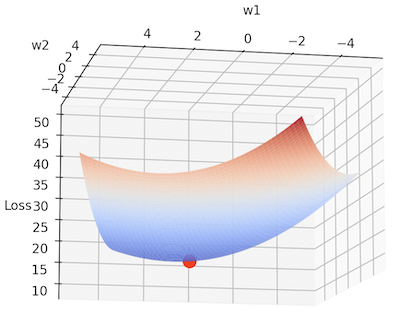 Gradient Descent finding global minima
This code generates synthetic data for a quadratic regression problem, initializes the model parameters, and performs gradient descent to find the values of the model parameters that minimize the mean squared error loss. The code also plots the loss surface and the trajectory of the gradient descent algorithm on the loss surface.
The resulting plot shows how the gradient descent algorithm takes small steps downhill on the loss surface and eventually reaches the global minimum of the loss function. The global minimum is the point on the loss surface where the loss is the lowest.
It is important to choose an appropriate learning rate for the gradient descent algorithm. If the learning rate is too small, the algorithm will take a long time to converge to the global minimum. On the other hand, if the learning rate is too large, the algorithm may overshoot the global minimum and may not converge to a good solution.
Another important consideration is the initialization of the model parameters. If the initialization is too far from the global minimum, the gradient descent algorithm may take a long time to converge. It is often helpful to initialize the model parameters to small random values.
It is also important to choose an appropriate stopping criterion for the gradient descent algorithm. One common stopping criterion is to stop the algorithm when the loss function stops improving or when the improvement is below a certain threshold. Another option is to stop the algorithm after a fixed number of iterations.
Overall, gradient descent is a powerful optimization algorithm that can be used to find the values of the model parameters that minimize the loss function for a wide range of machine learning problems.
Conclusion
In this blog, we have discussed gradient descent optimization in TensorFlow and how to implement it to train a linear regression model. We have seen that TensorFlow provides several optimizers that implement different variations of gradient descent, such as stochastic gradient descent and mini-batch gradient descent.
Gradient descent is a powerful optimization algorithm that is widely used in machine learning and deep learning to find the optimal solution to a given problem. It is an iterative algorithm that updates the parameters of a function by taking steps in the opposite direction of the gradient of the function. TensorFlow makes it easy to implement gradient descent by providing built-in optimizers and functions for computing gradients.
Similar Reads
Deep Learning Tutorial Deep Learning tutorial covers the basics and more advanced topics, making it perfect for beginners and those with experience. Whether you're just starting or looking to expand your knowledge, this guide makes it easy to learn about the different technologies of Deep Learning.Deep Learning is a branc
5 min read
Introduction to Deep Learning
Basic Neural Network
Activation Functions
Artificial Neural Network
Classification
Regression
Hyperparameter tuning
Introduction to Convolution Neural Network
Introduction to Convolution Neural NetworkConvolutional Neural Network (CNN) is an advanced version of artificial neural networks (ANNs), primarily designed to extract features from grid-like matrix datasets. This is particularly useful for visual datasets such as images or videos, where data patterns play a crucial role. CNNs are widely us
8 min read
Digital Image Processing BasicsDigital Image Processing means processing digital image by means of a digital computer. We can also say that it is a use of computer algorithms, in order to get enhanced image either to extract some useful information. Digital image processing is the use of algorithms and mathematical models to proc
7 min read
Difference between Image Processing and Computer VisionImage processing and Computer Vision both are very exciting field of Computer Science. Computer Vision: In Computer Vision, computers or machines are made to gain high-level understanding from the input digital images or videos with the purpose of automating tasks that the human visual system can do
2 min read
CNN | Introduction to Pooling LayerPooling layer is used in CNNs to reduce the spatial dimensions (width and height) of the input feature maps while retaining the most important information. It involves sliding a two-dimensional filter over each channel of a feature map and summarizing the features within the region covered by the fi
5 min read
CIFAR-10 Image Classification in TensorFlowPrerequisites:Image ClassificationConvolution Neural Networks including basic pooling, convolution layers with normalization in neural networks, and dropout.Data Augmentation.Neural Networks.Numpy arrays.In this article, we are going to discuss how to classify images using TensorFlow. Image Classifi
8 min read
Implementation of a CNN based Image Classifier using PyTorchIntroduction: Introduced in the 1980s by Yann LeCun, Convolution Neural Networks(also called CNNs or ConvNets) have come a long way. From being employed for simple digit classification tasks, CNN-based architectures are being used very profoundly over much Deep Learning and Computer Vision-related t
9 min read
Convolutional Neural Network (CNN) ArchitecturesConvolutional Neural Network(CNN) is a neural network architecture in Deep Learning, used to recognize the pattern from structured arrays. However, over many years, CNN architectures have evolved. Many variants of the fundamental CNN Architecture This been developed, leading to amazing advances in t
11 min read
Object Detection vs Object Recognition vs Image SegmentationObject Recognition: Object recognition is the technique of identifying the object present in images and videos. It is one of the most important applications of machine learning and deep learning. The goal of this field is to teach machines to understand (recognize) the content of an image just like
5 min read
YOLO v2 - Object DetectionIn terms of speed, YOLO is one of the best models in object recognition, able to recognize objects and process frames at the rate up to 150 FPS for small networks. However, In terms of accuracy mAP, YOLO was not the state of the art model but has fairly good Mean average Precision (mAP) of 63% when
7 min read
Recurrent Neural Network
Natural Language Processing (NLP) TutorialNatural Language Processing (NLP) is a branch of Artificial Intelligence (AI) that helps machines to understand and process human languages either in text or audio form. It is used across a variety of applications from speech recognition to language translation and text summarization.Natural Languag
5 min read
NLTK - NLPNatural Language Toolkit (NLTK) is one of the largest Python libraries for performing various Natural Language Processing tasks. From rudimentary tasks such as text pre-processing to tasks like vectorized representation of text - NLTK's API has covered everything. In this article, we will accustom o
5 min read
Word Embeddings in NLPWord Embeddings are numeric representations of words in a lower-dimensional space, that capture semantic and syntactic information. They play a important role in Natural Language Processing (NLP) tasks. Here, we'll discuss some traditional and neural approaches used to implement Word Embeddings, suc
14 min read
Introduction to Recurrent Neural NetworksRecurrent Neural Networks (RNNs) differ from regular neural networks in how they process information. While standard neural networks pass information in one direction i.e from input to output, RNNs feed information back into the network at each step.Imagine reading a sentence and you try to predict
10 min read
Recurrent Neural Networks ExplanationToday, different Machine Learning techniques are used to handle different types of data. One of the most difficult types of data to handle and the forecast is sequential data. Sequential data is different from other types of data in the sense that while all the features of a typical dataset can be a
8 min read
Sentiment Analysis with an Recurrent Neural Networks (RNN)Recurrent Neural Networks (RNNs) are used in sequence tasks such as sentiment analysis due to their ability to capture context from sequential data. In this article we will be apply RNNs to analyze the sentiment of customer reviews from Swiggy food delivery platform. The goal is to classify reviews
5 min read
Short term MemoryIn the wider community of neurologists and those who are researching the brain, It is agreed that two temporarily distinct processes contribute to the acquisition and expression of brain functions. These variations can result in long-lasting alterations in neuron operations, for instance through act
5 min read
What is LSTM - Long Short Term Memory?Long Short-Term Memory (LSTM) is an enhanced version of the Recurrent Neural Network (RNN) designed by Hochreiter and Schmidhuber. LSTMs can capture long-term dependencies in sequential data making them ideal for tasks like language translation, speech recognition and time series forecasting. Unlike
5 min read
Long Short Term Memory Networks ExplanationPrerequisites: Recurrent Neural Networks To solve the problem of Vanishing and Exploding Gradients in a Deep Recurrent Neural Network, many variations were developed. One of the most famous of them is the Long Short Term Memory Network(LSTM). In concept, an LSTM recurrent unit tries to "remember" al
7 min read
LSTM - Derivation of Back propagation through timeLong Short-Term Memory (LSTM) are a type of neural network designed to handle long-term dependencies by handling the vanishing gradient problem. One of the fundamental techniques used to train LSTMs is Backpropagation Through Time (BPTT) where we have sequential data. In this article we see how BPTT
4 min read
Text Generation using Recurrent Long Short Term Memory NetworkLSTMs are a type of neural network that are well-suited for tasks involving sequential data such as text generation. They are particularly useful because they can remember long-term dependencies in the data which is crucial when dealing with text that often has context that spans over multiple words
4 min read