ML | Logistic Regression using Tensorflow
Last Updated : 24 May, 2024
Prerequisites:
Understanding Logistic Regression and
TensorFlow.
Brief Summary of Logistic Regression: Logistic Regression is Classification algorithm commonly used in Machine Learning. It allows categorizing data into discrete classes by learning the relationship from a given set of labeled data. It learns a linear relationship from the given dataset and then introduces a non-linearity in the form of the Sigmoid function. In case of Logistic regression, the hypothesis is the Sigmoid of a straight line, i.e,
h(x) = \sigma(wx + b) where
\sigma(z) = \frac{1}{1 + e^{-z}} Where the vector
w represents the Weights and the scalar
b represents the Bias of the model. Let us visualize the Sigmoid Function -
Python3 import numpy as np import matplotlib.pyplot as plt def sigmoid(z): return 1 / (1 + np.exp( - z)) plt.plot(np.arange(-5, 5, 0.1), sigmoid(np.arange(-5, 5, 0.1))) plt.title('Visualization of the Sigmoid Function') plt.show() 
Note that the range of the Sigmoid function is (0, 1) which means that the resultant values are in between 0 and 1. This property of Sigmoid function makes it a really good choice of Activation Function for Binary Classification. Also
for z = 0, Sigmoid(z) = 0.5 which is the midpoint of the range of Sigmoid function. Just like Linear Regression, we need to find the optimal values of
w and
b for which the cost function
J is minimum. In this case, we will be using the Sigmoid Cross Entropy cost function which is given by
J(w, b) = -\frac{1}{m} \sum_{i=1}^{m}(y_i * log(h(x_i)) + (1 - y_i) * log(1 - h(x_i))) This cost function will then be optimized using Gradient Descent.
Implementation: We will start by importing the necessary libraries. We will use Numpy along with Tensorflow for computations, Pandas for basic Data Analysis and Matplotlib for plotting. We will also be using the preprocessing module of
Scikit-Learn for One Hot Encoding the data.
Python3 # importing modules import numpy as np import pandas as pd import tensorflow as tf import matplotlib.pyplot as plt from sklearn.preprocessing import OneHotEncoder
Next we will be importing the
dataset. We will be using a subset of the famous
Iris dataset.
Python3 data = pd.read_csv('dataset.csv', header = None) print("Data Shape:", data.shape) print(data.head()) Data Shape: (100, 4) 0 1 2 3 0 0 5.1 3.5 1 1 1 4.9 3.0 1 2 2 4.7 3.2 1 3 3 4.6 3.1 1 4 4 5.0 3.6 1
Now let's get the feature matrix and the corresponding labels and visualize.
Python3 # Feature Matrix x_orig = data.iloc[:, 1:-1].values # Data labels y_orig = data.iloc[:, -1:].values print("Shape of Feature Matrix:", x_orig.shape) print("Shape Label Vector:", y_orig.shape) Shape of Feature Matrix: (100, 2) Shape Label Vector: (100, 1)
Visualize the given data.
Python3 # Positive Data Points x_pos = np.array([x_orig[i] for i in range(len(x_orig)) if y_orig[i] == 1]) # Negative Data Points x_neg = np.array([x_orig[i] for i in range(len(x_orig)) if y_orig[i] == 0]) # Plotting the Positive Data Points plt.scatter(x_pos[:, 0], x_pos[:, 1], color = 'blue', label = 'Positive') # Plotting the Negative Data Points plt.scatter(x_neg[:, 0], x_neg[:, 1], color = 'red', label = 'Negative') plt.xlabel('Feature 1') plt.ylabel('Feature 2') plt.title('Plot of given data') plt.legend() plt.show() 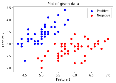
. Now we will be One Hot Encoding the data for it to work with the algorithm. One hot encoding transforms categorical features to a format that works better with classification and regression algorithms. We will also be setting the Learning Rate and the number of Epochs.
Python3 # Creating the One Hot Encoder oneHot = OneHotEncoder() # Encoding x_orig oneHot.fit(x_orig) x = oneHot.transform(x_orig).toarray() # Encoding y_orig oneHot.fit(y_orig) y = oneHot.transform(y_orig).toarray() alpha, epochs = 0.0035, 500 m, n = x.shape print('m =', m) print('n =', n) print('Learning Rate =', alpha) print('Number of Epochs =', epochs) m = 100 n = 7 Learning Rate = 0.0035 Number of Epochs = 500
Now we will start creating the model by defining the placeholders
X and
Y, so that we can feed our training examples
x and
y into the optimizer during the training process. We will also be creating the trainable Variables
W and
b which can be optimized by the Gradient Descent Optimizer.
Python3 # There are n columns in the feature matrix # after One Hot Encoding. X = tf.placeholder(tf.float32, [None, n]) # Since this is a binary classification problem, # Y can take only 2 values. Y = tf.placeholder(tf.float32, [None, 2]) # Trainable Variable Weights W = tf.Variable(tf.zeros([n, 2])) # Trainable Variable Bias b = tf.Variable(tf.zeros([2]))
Now declare the Hypothesis, Cost function, Optimizer and Global Variables Initializer.
Python3 # Hypothesis Y_hat = tf.nn.sigmoid(tf.add(tf.matmul(X, W), b)) # Sigmoid Cross Entropy Cost Function cost = tf.nn.sigmoid_cross_entropy_with_logits( logits = Y_hat, labels = Y) # Gradient Descent Optimizer optimizer = tf.train.GradientDescentOptimizer( learning_rate = alpha).minimize(cost) # Global Variables Initializer init = tf.global_variables_initializer()
Begin the training process inside a Tensorflow Session.
Python3 # Starting the Tensorflow Session with tf.Session() as sess: # Initializing the Variables sess.run(init) # Lists for storing the changing Cost and Accuracy in every Epoch cost_history, accuracy_history = [], [] # Iterating through all the epochs for epoch in range(epochs): cost_per_epoch = 0 # Running the Optimizer sess.run(optimizer, feed_dict = {X : x, Y : y}) # Calculating cost on current Epoch c = sess.run(cost, feed_dict = {X : x, Y : y}) # Calculating accuracy on current Epoch correct_prediction = tf.equal(tf.argmax(Y_hat, 1), tf.argmax(Y, 1)) accuracy = tf.reduce_mean(tf.cast(correct_prediction, tf.float32)) # Storing Cost and Accuracy to the history cost_history.append(sum(sum(c))) accuracy_history.append(accuracy.eval({X : x, Y : y}) * 100) # Displaying result on current Epoch if epoch % 100 == 0 and epoch != 0: print("Epoch " + str(epoch) + " Cost: " + str(cost_history[-1])) Weight = sess.run(W) # Optimized Weight Bias = sess.run(b) # Optimized Bias # Final Accuracy correct_prediction = tf.equal(tf.argmax(Y_hat, 1), tf.argmax(Y, 1)) accuracy = tf.reduce_mean(tf.cast(correct_prediction, tf.float32)) print("\nAccuracy:", accuracy_history[-1], "%") Epoch 100 Cost: 125.700202942 Epoch 200 Cost: 120.647117615 Epoch 300 Cost: 118.151592255 Epoch 400 Cost: 116.549999237 Accuracy: 91.0000026226 %
Let's plot the change of cost over the epochs.
Python3 plt.plot(list(range(epochs)), cost_history) plt.xlabel('Epochs') plt.ylabel('Cost') plt.title('Decrease in Cost with Epochs') plt.show() 
Plot the change of accuracy over the epochs.
Python3 plt.plot(list(range(epochs)), accuracy_history) plt.xlabel('Epochs') plt.ylabel('Accuracy') plt.title('Increase in Accuracy with Epochs') plt.show() 
Now we will be plotting the Decision Boundary for our trained classifier. A decision boundary is a hypersurface that partitions the underlying vector space into two sets, one for each class.
Python3 # Calculating the Decision Boundary decision_boundary_x = np.array([np.min(x_orig[:, 0]), np.max(x_orig[:, 0])]) decision_boundary_y = (- 1.0 / Weight[0]) * (decision_boundary_x * Weight + Bias) decision_boundary_y = [sum(decision_boundary_y[:, 0]), sum(decision_boundary_y[:, 1])] # Positive Data Points x_pos = np.array([x_orig[i] for i in range(len(x_orig)) if y_orig[i] == 1]) # Negative Data Points x_neg = np.array([x_orig[i] for i in range(len(x_orig)) if y_orig[i] == 0]) # Plotting the Positive Data Points plt.scatter(x_pos[:, 0], x_pos[:, 1], color = 'blue', label = 'Positive') # Plotting the Negative Data Points plt.scatter(x_neg[:, 0], x_neg[:, 1], color = 'red', label = 'Negative') # Plotting the Decision Boundary plt.plot(decision_boundary_x, decision_boundary_y) plt.xlabel('Feature 1') plt.ylabel('Feature 2') plt.title('Plot of Decision Boundary') plt.legend() plt.show() 