Probability Distribution - Function, Formula, Table

Last Updated : 22 May, 2025

A probability distribution is a mathematical function or rule that describes how the probabilities of different outcomes are assigned to the possible values of a random variable. It provides a way of modeling the likelihood of each outcome in a random experiment.

While a frequency distribution shows how often outcomes occur in a sample or dataset, a probability distribution assigns probabilities to outcomes abstractly, theoretically, regardless of any specific dataset. These probabilities represent the likelihood of each outcome occurring.

Probability-Distribution-01 — Probability Distribution

In a discrete probability distribution, the random variable takes distinct values (like the outcome of rolling a die). In a continuous probability distribution, the random variable can take any value within a certain range (like the height of a person).

Key properties of a probability distribution include:

The probability of each outcome is greater than or equal to zero.
The sum of the probabilities of all possible outcomes equals 1.

Also Read: Frequency Distribution

Table of Content

Random Variables

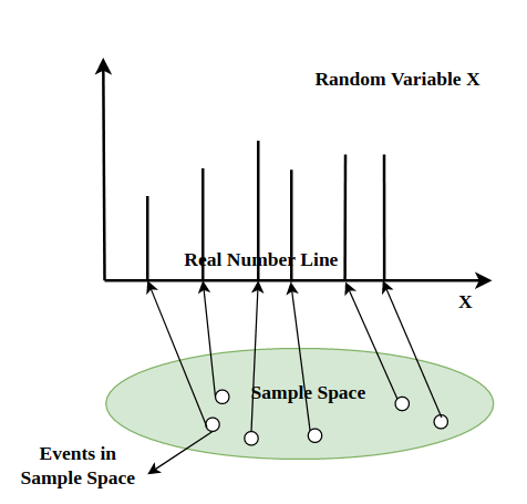
Random Variable is a real-valued function whose domain is the sample space of the random experiment. It is represented as X(sample space) = Real number.

We need to learn the concept of Random Variables because sometimes we are only interested in the probability of the event, but also the number of events associated with the random experiment. The importance of random variables can be better understood by the following example:

Let's take an example of the coin flips. We'll start with flipping a coin and finding out the probability. We'll use H for 'heads' and T for 'tails'.
So now we flip our coin 3 times, and we want to answer some questions.

What is the probability of getting exactly 3 heads?
What is the probability of getting less than 3 heads?
What is the probability of getting more than 1 head?

Then our general way of writing would be:

P(Probability of getting exactly 3 heads when we flip a coin 3 times)
P(Probability of getting less than 3 heads when we flip a coin 3 times)
P(Probability of getting more than 1 head when we flip a coin 3 times)

In a different scenario, suppose we are tossing two dice, and we are interested in knowing the probability of getting two numbers such that their sum is 6.

So, in both of these cases, we first need to know the number of times the desired event is obtained i.e. Random Variable X in sample space which would be then further used to compute the Probability P(X) of the event. Hence, Random Variables come to our rescue. First, let's define what is random variable mathematically.

A random variable is a real valued function whose domain is the sample space of a random experiment

To understand this concept in a lucid manner, let us consider the experiment of tossing a coin two times in succession.

The sample space of the experiment is S = {HH, HT, TH, TT}. Let's define a random variable to count events of heads or tails according to our need, Let X be a random variable that denotes the number of heads obtained. For each outcome, its values are as given below:

X(HH) = 2, X (HT) = 1, X (TH) = 1, X (TT) = 0.

More than one random variable can be defined in the same sample space. For example, let Y be a random variable denoting the number of heads minus the number of tails for each outcome of the above sample space S.

Y(HH) = 2 - 0 = 2; Y (HT) = 1 - 1 = 0; Y (TH) = 1 - 1 = 0; Y (TT) = 0 - 2 = – 2

Thus, X and Y are two different random variables defined on the same sample.

Note: More than one event can map to same value of random variable.

Types of Random Variables in Probability Distribution

There are the following two types of Random Variables:

Discrete Random Variables
Continuous Random Variables

Discrete Random Variables in Probability Distribution

A Discrete Random Variable can only take a finite number of values. To further understand this, let's see some examples of discrete random variables:

\sum_{i} P(X = x_i) = 1

X = {sum of the outcomes when two dice are rolled}. Here, X can only take values like {2, 3, 4, 5, 6, 10, 11, 12}.
X = {Number of Heads in 100 coin tosses}. Here, X can take only integer values from [0, 100].

Continuous Random Variable in Probability Distribution

A Continuous Random Variable can take infinite values in a continuous domain.

P(a \leq X \leq b) = \int_{a}^{b} f(x) \, dx

Let's see an example of a dart game.

Suppose, we have a dart game in which we throw a dart where the dart can fall anywhere between [-1, 1] on the x-axis. So if we define our random variable as the x-coordinate of the position of the dart, X can take any value from [-1, 1]. There are infinitely many possible values that X can take. (X = {0.1, 0.001, 0.01, 1, 2, 2.112121 .... and so on}.

Probability Distribution of a Random Variable

Now the question comes, how to describe the behavior of a random variable?

Suppose that our Random Variable only takes finite values, like x₁, x₂, x₃,..., and x_n. i.e., the range of X is the set of n values is {x₁, x₂, x₃,..., and x_n}.
Thus, the behavior of X is completely described by giving probabilities for all the values of the random variable X

Event	Probability
x₁	P(X = x₁)
x₂	P(X = x₂)
x₃	P(X = x₃)

The Probability Function of a discrete random variable X is the function p(x) satisfying.

P(x) = P(X = x)

Example: We draw two cards successively with replacement from a well-shuffled deck of 52 cards. Find the probability distribution of finding aces.

Answer:

Let's define a random variable "X", which means number of aces. So since we are only drawing two cards from the deck, X can only take three values: 0, 1 and 2. We also know that, we are drawing cards with replacement which means that the two draws can be considered an independent experiments.
P(X = 0) = P(both cards are non-aces)
= P(non-ace) x P(non-ace)
= \dfrac{48}{52} \times \dfrac{48}{52} = \dfrac {144}{169}
P(X = 1) = P(one of the cards in ace)
= P(non-ace and then ace) + P(ace and then non-ace)
= P(non-ace) x P(ace) + P(ace) x P(non-ace)
= \dfrac{48}{52} \times \dfrac{4}{52} + \dfrac{4}{52} \times \dfrac{48}{52} = \dfrac{24}{169}
P(X = 2) = P(Both the cards are aces)
= P(ace) x P(ace)
= \dfrac{4}{52} \times \dfrac{4}{52} = \dfrac{1}{169}
Now we have probabilities for each value of random variable. Since it is discrete, we can make a table to represent this distribution. The table is given below.

X	0	1	2
P(X = x)	144/169	24/169	1/169

It should be noted here that each value of P(X = x) is greater than zero and the sum of all P(X = x) is equal to 1.

Probability Distribution Formulas

The various formulas under Probability Distribution are tabulated below:

Types of Distribution

Formula

Binomial Distribution

P(X) = ⁿC_xa^xb^n-x

Where a = probability of success

b = probability of failure
n = number of trials
x = random variable denoting success

Cumulative Distribution Function

F_x(x) = \int_{-∞}^{x}f(x)(t)dt

Discrete Probability Distribution

P(x) = n!/ r!(n-r)! . p^r(1-p)^n-r
P(x) = C(n,r) . p^r(1-p)^n-r

Expectation (Mean) and Variance of a Random Variable

Suppose we have a probability experiment we are performing, and we have defined some random variable(R.V.) according to our needs( like we did in some previous examples). Now, each time an experiment is performed, our R.V. takes on a different value. But we want to know that if we keep on experimenting a thousand times or an infinite number of times, what will be the average value of the random variable?

Expectation

The mean, expected value, or expectation of a random variable X is written as E(X) or\mu_{\textbf{X}}. If we observe N random values of X, then the mean of the N values will be approximately equal to E(X) for large N.

For a random variable X which takes on values x₁, x_2,x_{3 ...}x_n with probabilities p₁, p₂, p₃ ... p_n. Expectation of X is defined as,
\sum_{i=1}^{N} x_{i}p_{i}
i.e it is weighted average of all values which X can take, weighted by the probability of each value.

To see it more intuitively, let's take a look at this graph below,

Now, in the above figure, we can see both the Random Variables have almost the same 'mean', but does that mean that they are equal? No. To fully describe the properties/behavior of a random variable, we need something more, right?

We need to look at the dispersion of the probability distribution, one of them is concentrated, but the other is very spread out near a single value. So we need a metric to measure the dispersion in the graph.

Variance

In Statistics, we have studied that the variance is a measure of the spread or scatter in the data. Likewise, the variability or spread in the values of a random variable may be measured by variance.

For a random variable X which takes on values x₁, x₂, x₃ ... x_n with probabilities p₁, p₂, p₃ ... p_n and the expectation is E[X]
The variance of X or Var(X) is denoted by, E[X - u]^{2} = \sum (x_{i}-\mu)^{2}p_{x_{i}} = E[X^{2}] - (E[X])^{2}

Example: Find the variance and mean of the numbers obtained on a throw of an unbiased die.

Answer:

We know that the sample space of this experiment is {1, 2, 3, 4, 5, 6}
Let's define our random variable X, which represents the number obtained on a throw.
So, the probabilities of the values which our random variable can take are,
P(1) = P(2) = P(3) = P(4) = P(5) = P(6) = 1/6
Therefore, the probability distribution of the random variable is,
X 1 2 3 4 5 6
Probabilities 1/6 1/6 1/6 1/6 1/6 1/6
E[X] = \sum p_{x_{i}}x_{i} \\ \hspace{0.9cm} = 1 \times \dfrac{1}{6} + 2 \times \dfrac{1}{6} + 3 \times \dfrac{1}{6} + 4 \times \dfrac{1}{6} + 5 \times \dfrac{1}{6} + 6 \times \dfrac{1}{6} \\ \hspace{0.9cm} = \dfrac{21}{6}
Also, E[X²] = 1^{2} \times \dfrac{1}{6} + 2^{2}\times\dfrac{1}{6} + 3^{2}\times\dfrac{1}{6} + 4^{2}\times\dfrac{1}{6} + 5^{2}\times\dfrac{1}{6} + 6^{2}\times\dfrac{1}{6} \\ \hspace{0.9cm} = \dfrac{91}{6} \\
Thus, Var(X) = E[X²] - (E[X])²
= (\dfrac{91}{6}) - (\dfrac{21}{6})^{2} = \dfrac{91}{6} - \dfrac{441}{36} = \dfrac{35}{12}
So, therefore mean is \dfrac{21}{6}and variance is \dfrac{35}{12}

Different Types of Probability Distributions

We have seen what Probability Distributions are, now we will see different types of Probability Distributions. The Probability Distribution's type is determined by the type of random variable. There are two types of Probability Distributions:

Binomial or Discrete Probability Distributions for Discrete Variables
Normal or Cumulative Probability Distribution for continuous variables

We will study in detail two types of discrete probability distributions, others are out of scope in class 12.

Discrete Probability Distributions

Discrete Probability Functions also called Binomial Distribution assume a discrete number of values. For example, coin tosses and counts of events are discrete functions. These are discrete distributions because there are no in-between values. We can either have heads or tails in a coin toss.

For discrete probability distribution functions, each possible value has a non-zero probability. Moreover, the sum of all the values of probabilities must be one. For example, the probability of rolling a specific number on a die is 1/6. The total probability for all six values equals one. When we roll a die, we only get either one of these values.

Bernoulli Trials and Binomial Distributions

When we perform a random experiment, either we get the desired event or we don't. If we get the desired event, then we call it a success, and if we don't it is a failure. Let's say in the coin-tossing experiment, if the occurrence of the head is considered a success, then the occurrence of a tail is a failure.

Each time we toss a coin or roll a die or perform any other experiment, we call it a trial. Now we know that in our experiments coin-tossing trial, the outcome of any trial is independent of the outcome of any other trial. In each of such trials, the probability of success or failure remains constant. Such independent trials that have only two outcomes, usually referred to as ‘success’ or ‘failure’, are called Bernoulli Trials.

Definition:

Trials of the random experiment are known as Bernoulli Trials, if they are satisfying below given conditions :
Finite number of trials are required.
All trials must be independent.
Every trial has two outcomes : success or failure.
Probability of success remains same in every trial.

Example 1: Can throwing a fair die 50 times be considered an example of 50 Bernoulli trials if we define:

Success is getting an even number (2, 4, or 6), and
Failure as getting an odd number (1, 3, or 5)?

If yes, what are the probabilities of success (p) and failure (q) for each trial?

Answer:

Probability of Success (p): There are 3 even numbers out of 6 possible outcomes, so p = 3/6 = 1 /2
Probability of Failure (q): There are 3 odd numbers out of 6, so q = 3/6 = 1 /2
So, throwing a fair die 50 times with this definition is a classic example of 50 Bernoulli trials, with p=1/2 and q = 1/2

Example 2: An urn contains 8 red balls and 10 black balls. We draw six balls from the urn successively. You have to tell whether or not the trials of drawing balls are Bernoulli trials when, after each draw, the ball drawn is:

Replaced
Not replaced in the urn.

Answer:

We know that the number of trials are finite. When drawing is done with replacement, probability of success (say, red ball) is p =8/18 which will be same for all of the six trials. So, drawing of balls with replacements are Bernoulli trials.
If drawing is done without replacement, probability of success (i.e., red ball) in the first trial is 8/18 , in 2nd trial is 7/17 if first ball drawn is red or, 10/18 if first ball drawn is black, and so on. Clearly, probabilities of success are not same for all the trials, Therefore, the trials are not Bernoulli trials.

Binomial Distribution

It is a random variable that represents the number of successes in "N" successive independent trials of Bernoulli's experiment. It is used in a plethora of instances including the number of heads in "N" coin flips, and so on.

Let P and Q denote the success and failure of the Bernoulli Trial respectively. Let's assume we are interested in finding different ways in which we have 1 success in all six trials.
Six cases are available as listed below:

PQQQQQ, QPQQQQ, QQPQQQ, QQQPQQ, QQQQPQ, QQQQQP

Likewise, 2 successes and 4 failures will show \dfrac{6!}{4! 2!}combinations thus making it difficult to list so many combinations. Henceforth, calculating probabilities of 0, 1, 2,..., n number of successes can be long and time-consuming. To avoid such lengthy calculations along with a listing of all possible cases, for probabilities of the number of successes in n-Bernoulli trials, a formula is made which is given as:

If Y is a Binomial Random Variable, we denote this Y∼ Bin(n, p), where p is the probability of success in a given trial, q is the probability of failure, Let 'n' be the total number of trials, and 'x' be the number of successes, the Probability Function P(Y) for Binomial Distribution is given as:

P(Y) = ⁿC_x q^n–xp^x
where x = 0,1,2...n

Example: When a fair coin is tossed 10 times, find the probability of getting:

Exactly Six Heads
At least Six Heads

Answer:

Every coin tossed can be considered as the Bernoulli trial. Suppose X is the number of heads in this experiment:
We already know, n = 10
p = 1/2
So, P(X = x) = ⁿC_x p^n-x (1-p)^x, x= 0,1,2,3,....n
P(X = x) = ¹⁰C_xp^10-x(1-p)^x
When x = 6,
(i) P(x = 6) = ¹⁰C₆ p⁴ (1-p)⁶
= \dfrac{10!}{6!4!}(\dfrac{1}{2})^{6}(\dfrac{1}{2})^{4}\\ \hspace{0.4cm} = \dfrac{7\times8\times9\times10}{2\times3\times4}\times\dfrac{1}{64}\times\dfrac{1}{16} \\ \hspace{0.4cm} = \dfrac{105}{512}
(ii) P(at least 6 heads) = P(X >= 6) = P(X = 6) + P(X=7) + P(X=8)+ P(X=9) + P(X=10)
= ¹⁰C₆ p⁴(1 - p)⁶+ ¹⁰C₇p³(1 - p)⁷ + ¹⁰C₈p²(1 - p)⁸+ ¹⁰C₉p¹(1 - p)⁹ + ¹⁰C₁₀(1 - p)¹⁰
=\dfrac{10!}{6!4!}(\dfrac{1}{2})^{10} + \dfrac{10!}{7!3!}(\dfrac{1}{2})^{10} + \dfrac{10!}{8!2!}(\dfrac{1}{2})^{10} + \dfrac{10!}{9!1!}(\dfrac{1}{2})^{10} + \dfrac{10!}{10!}(\dfrac{1}{2})^{10}\\ \hspace{0.5cm} = (\dfrac{10!}{6!4!} + \dfrac{10!}{7!3!}+ \dfrac{10!}{8!2!} + \dfrac{10!}{9!1!}+ \dfrac{10!}{10!})(\dfrac{1}{2})^{10} \\ \hspace{0.5cm} = \dfrac{193}{512}

Negative Binomial Distribution

In a random experiment of a discrete range, we don't need to get success in every trial. If we perform the 'n' number of trials and get success 'r' times where n > r, then our failure will be (n - r) times. The probability distribution of failure in this case will be called the negative binomial distribution.
For example, if we consider getting 6 in the die is a success and we want 6 one time, but 6 is not obtained in the first trial then we keep throwing the die until we get 6. Suppose we get 6 in the sixth trial then the first 5 trials will be failures and if we plot the probability distribution of these failures, then the plot so obtained will be called a negative binomial distribution.

Poisson Probability Distribution

The Probability Distribution of the frequency of occurrence of an event over a specific period is called the Poisson Distribution. It tells how many times the event occurred over a specific period. It counts the number of successes and takes a value of the whole number i.e., (0,1,2...). It is expressed as

f(x; λ) = P(X = x) = (λ^xe^-λ)/x!

where,

x is the number of times the event occurred
e = 2.718...
λ is the mean value

Binomial Distribution Examples

Binomial Distribution is used for the outcomes that are discrete in nature. Some of the examples where the Binomial Distribution can be used are mentioned below:

To find the number of good and defective items produced by a factory.
To find the number of girls and boys studying in a school.
To find out the negative or positive feedback on something

Cumulative Probability Distribution

The Cumulative Probability Distribution for continuous variables is a function that gives the probability that a random variable takes on a value less than or equal to a specified point. It's denoted as F(x), where x represents a specific value of the random variable. For continuous variables, F(x) is found by integrating the probability density function (pdf) from negative infinity to x. The function ranges from 0 to 1, is non-decreasing, and right-continuous. It's essential for computing probabilities, determining percentiles, and understanding the behavior of continuous random variables in various fields.

Cumulative Probability Distribution takes values in a continuous range; for example, the range may consist of a set of real numbers. In this case, the Cumulative Probability Distribution will take any value from the continuum of real numbers unlike the discrete or some finite value taken in the case of Discrete Probability distribution. Cumulative Probability Distribution is of two types, Continuous Uniform Distributionthe and Normal Distribution.

Continuous Uniform Distribution

Continuous Uniform Distribution is described by a density function that is flat and assumes values in a closed interval let's say [P, Q], such that the probability is uniform in this closed interval. It is represented as f(x; P, Q)

f(x; P, Q) = 1/(Q - P) for P ≤ x ≤ Q
f(x; P, Q) = 0; elsewhere

Normal Distribution

Normal Distribution of continuous random variables results in a bell-shaped curve. It is often referred to as the Gaussian Distribution by the name of Karl Friedrich Gauss who derived its equation. This curve is frequently used by the meteorological department for rainfall studies. The Normal Distribution of random variable X is given by

n(x; μ, σ) = {1/(√2π)σ}e^{(-1/2σ^2)(x-μ)^2} for -∞<x<∞

where

μ is the mean
σ is variance

Normal Distribution Examples

The Normal Distribution Curve can be used to show the distribution of natural events very well. Over the period, it has become a favorite choice of statisticians to study natural events. Some of the examples where the Normal Distribution Curve can be used are mentioned below.

Salary of the Working Class
Life Expectancy of humans in a Country
Heights of Male or Female
The IQ Level of Children
Expenditure of households

Probability Distribution Function

Probability Distribution Function is defined as the function that is used to express the distribution of a probability. Different types of probability, are expressed differently. These functions are also used for Probability Density Functions for different variables.

For Normal Distribution, the Probability Distribution Function for Random Variable X is given by F_x(x) = P(X ≤ x) where X is the Random variable and P is the Probability.

The Cumulative Probability Distribution for closed interval a⇢b is given as P(a < X ≤ b) = F_x(b) - F_x(a).

In terms of integrals, the cumulative probability function is given as F_{x}(x) = \int_{-\infty }^{x}f_{x}(t)dt

For Random Variable X = p, the Cumulative Probability function is given as P(X = p) = F_{x}(p) - \lim_{x\rightarrow p}f_{x}(t)

Binomial Probability Distribution gives some exact values. It is often called a Probability Mass Function. For a Random Variable X and Space S where X: S⇢A where A belongs to Random Discrete Variable R, X can be defined as f_x(x) = P_r(X = x) = P({s ∈ S: X(s) = x}).

Probability Distribution Table

The random variables and their corresponding probability is tabulated, then it is called a Probability Distribution Table. The following table represents a Probability Distribution Table:

X	X₁	X₂	X₃	X₄	....	X_n
P(X)	P₁	P₂	P₃	P₄	....	P_n

It should be noted that the sum of all probabilities is equal to 1.

Prior Probability

Prior Probability as the name suggests refers to assigning the probability of an event before the happening of a dependent event which makes us make changes in the Prior Probability. Let's say we assign Probability P(A) to event A before taking into account that event B has also happened. After B has happened we need to revise P(A) using Bayes' Theorem. Hence, here P(A) is the Prior Probability. If we predict that a particular observation will fall into a particular category before collecting all the observations, then this is also called Prior Probability.

Posterior Probability

After the Prior Probability has been assigned and new information is obtained then the Prior Probability is modified by taking into account the newly obtained information using Baye's Formula. This revised probability is called Posterior Probability. Hence, we can say that Posterior Probability is a conditional probability obtained by revising the Prior Probability.

Chi-Square Distribution

The chi-square distribution is a probability distribution that arises in statistics, particularly in hypothesis testing and confidence interval estimation. It is characterized by its degrees of freedom, which determine its shape. The distribution is positively skewed and only takes non-negative values. The Chi-square distribution is widely used in inferential statistics for testing the independence of variables in contingency tables, assessing goodness of fit, and estimating population variances.

Chi-Square Table

Below is a Chi-square table showing critical values for selected degrees of freedom and levels of significance:

Degrees of Freedom (df)	0.01	0.05	0.10
1	6.63	3.84	2.71
2	9.21	5.99	4.61
3	11.34	7.81	6.25
4	13.28	9.49	7.78
5	15.09	11.07	9.24
6	16.81	12.59	10.64
7	18.48	14.07	12.02
8	20.09	15.51	13.36
9	21.67	16.92	14.68
10	23.21	18.31	15.99

This table provides critical values for the Chi-square distribution at various levels of significance (0.01, 0.05, and 0.10) and degrees of freedom (from 1 to 10). Critical values from the Chi-square table are commonly used in hypothesis testing to determine whether observed frequencies in a contingency table differ significantly from expected frequencies.

t-Distribution

The t distribution, also known as the Student's t-distribution, is a probability distribution that is similar to the standard normal distribution but has heavier tails. It is commonly used in hypothesis testing and constructing confidence intervals when the sample size is small or the population standard deviation is unknown. The shape of the t distribution depends on the sample size, and as the sample size increases, the t-distribution approaches the standard normal distribution.

t-Table

Below is a t-table showing critical values for selected degrees of freedom (df) and levels of significance:

Degrees of Freedom (df)	0.01	0.05	0.10
1	12.706	6.314	3.078
2	4.303	2.920	1.886
3	3.182	2.353	1.638
4	2.776	2.132	1.533
5	2.571	2.015	1.476
6	2.447	1.943	1.440
7	2.365	1.895	1.415
8	2.306	1.860	1.397
9	2.262	1.833	1.383
10	2.228	1.812	1.372

This table provides critical values for the t-distribution at various levels of significance (0.01, 0.05, and 0.10) and degrees of freedom (from 1 to 10). Critical values from the t-table are commonly used in hypothesis testing to determine whether sample means significantly differ from population means when the population standard deviation is unknown and sample sizes are small.

Solved Questions on Probability Distribution

Question 1: A box contains 4 blue balls and 3 green balls. Find the probability distribution of the number of green balls in a random draw of 3 balls.

Solution:

Given that the total number of balls is 7 out of which 3 have to be drawn at random. On drawing 3 balls the possibilities are all 3 are green, only 2 is green, only 1 is green, and no green. Hence X = 0, 1, 2, 3.
P(No ball is green) = P(X = 0) = ⁴C₃/⁷C₃ = 4/35
P(1 ball is green) = P(X = 1) = ³C₁ × ⁴C₂/ ⁷C₃ = 18/35
P(2 balls are green) = P(X = 2) = ³C₂ × ⁴C₁/ ⁷C₃ = 12/35
P(All 3 balls are green) = P(X = 3) = ³C₃/ ⁷C₃ = 1/35
Hence, the probability distribution for this problem is given as follows
X 0 1 2 3
P(X) 4/35 18/35 12/35 1/35

Question 2: From a lot of 10 bulbs containing 3 defective ones, 4 bulbs are drawn at random. If X is a random variable that denotes the number of defective bulbs. Find the probability distribution of X.

Solution:

Since, X denotes the number of defective bulbs and there is a maximum of 3 defective bulbs, hence X can take values 0, 1, 2, and 3. Since 4 bulbs are drawn at random, the possible combination of drawing 4 bulbs is given by 10C4.
P(Getting No defective bulb) = P(X = 0) = ⁷C₄/ ¹⁰C₄ = 1/6
P(Getting 1 Defective Bulb) = P(X = 1) = ³C₁ × ⁷C₃/¹⁰C₄ = 1/2
P(Getting 2 defective Bulb) = P(X = 2) = ³C₂ × ⁷C₂/¹⁰C₄ = 3/10
P(Getting 3 Defective Bulb) = P(X = 3) = ³C₃ × ⁷C₁/¹⁰C₄ = 1/30
Hence Probability Distribution Table is given as follows
X 0 1 2 3
P(X) 1/6 1/2 3/10 1/30

Articles related to Probability Distribution
Probability Theory	Probability Density Function
Types of Events in Probability	Events in Probability

Descriptive Statistic

anjalishukla1859

Improve

Article Tags :

Probability Distribution - Function, Formula, Table

Random Variables

Types of Random Variables in Probability Distribution

Discrete Random Variables in Probability Distribution

Continuous Random Variable in Probability Distribution

Probability Distribution of a Random Variable

Probability Distribution Formulas

Expectation (Mean) and Variance of a Random Variable

Expectation

Variance

Different Types of Probability Distributions

Discrete Probability Distributions

Bernoulli Trials and Binomial Distributions

Binomial Distribution

Negative Binomial Distribution

Poisson Probability Distribution

Binomial Distribution Examples

Cumulative Probability Distribution

Continuous Uniform Distribution

Normal Distribution

Probability Distribution Function

Probability Distribution Table

Prior Probability

Posterior Probability

Chi-Square Distribution

Chi-Square Table

t-Distribution

t-Table

Solved Questions on Probability Distribution

Articles related to Probability Distribution

Similar Reads

Basic Arithmetic

Algebra

Geometry

Trigonometry & Vector Algebra

Calculus

Probability and Statistics

Practice