Gated Recurrent Unit Networks

Last Updated : 04 Jun, 2025

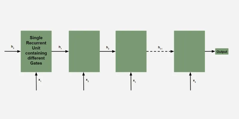
In machine learning Recurrent Neural Networks (RNNs) are essential for tasks involving sequential data such as text, speech and time-series analysis. While traditional RNNs struggle with capturing long-term dependencies due to the vanishing gradient problem architectures like Long Short-Term Memory (LSTM) networks were developed to overcome this limitation.

However LSTMs are very complex structure with higher computational cost. To overcome this Gated Recurrent Unit (GRU) where introduced which uses LSTM architecture by merging its gating mechanisms offering a more efficient solution for many sequential tasks without sacrificing performance. In this article we'll learn more about them.

What are Gated Recurrent Units (GRU) ?

Gated Recurrent Units (GRUs) are a type of RNN introduced by Cho et al. in 2014. The core idea behind GRUs is to use gating mechanisms to selectively update the hidden state at each time step allowing them to remember important information while discarding irrelevant details. GRUs aim to simplify the LSTM architecture by merging some of its components and focusing on just two main gates: the update gate and the reset gate.

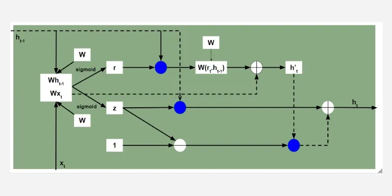
The GRU consists of two main gates:

Update Gate (z_t): This gate decides how much information from previous hidden state should be retained for the next time step.
Reset Gate (r_t): This gate determines how much of the past hidden state should be forgotten.

These gates allow GRU to control the flow of information in a more efficient manner compared to traditional RNNs which solely rely on hidden state.

Equations for GRU Operations

The internal workings of a GRU can be described using following equations:

1. Reset gate:

r_t = \sigma \left( W_r \cdot [h_{t-1}, x_t] \right)

The reset gate determines how much of the previous hidden state h_{t-1} should be forgotten.

2. Update gate:

z_t = \sigma(W_z \cdot [h_{t-1}, x_t])

The update gate controls how much of the new information x_t should be used to update the hidden state.

3. Candidate hidden state:

h_t' = \tanh(W_h \cdot [r_t \cdot h_{t-1}, x_t])

This is the potential new hidden state calculated based on the current input and the previous hidden state.

4. Hidden state:

h_t = (1 - z_t) \cdot h_{t-1} + z_t \cdot h_t'

The final hidden state is a weighted average of the previous hidden state h_{t-1} and the candidate hidden state h_t' based on the update gate z_t.

How GRUs Solve the Vanishing Gradient Problem

Like LSTMs, GRUs were designed to address the vanishing gradient problem which is common in traditional RNNs. GRUs help mitigate this issue by using gates that regulate the flow of gradients during training ensuring that important information is preserved and that gradients do not shrink excessively over time. By using these gates, GRUs maintain a balance between remembering important past information and learning new, relevant data.

GRU vs LSTM

GRUs are more computationally efficient because they combine the forget and input gates into a single update gate. GRUs do not maintain an internal cell state as LSTMs do, instead they store information directly in the hidden state making them simpler and faster.

Feature	LSTM (Long Short-Term Memory)	GRU (Gated Recurrent Unit)
Gates	3 (Input, Forget, Output)	2 (Update, Reset)
Cell State	Yes it has cell state	No (Hidden state only)
Training Speed	Slower due to complexity	Faster due to simpler architecture
Computational Load	Higher due to more gates and parameters	Lower due to fewer gates and parameters
Performance	Often better in tasks requiring long-term memory	Performs similarly in many tasks with less complexity

Implementation in Python

Now let's implement simple GRU model in Python using Keras. We'll start by preparing the necessary libraries and dataset.

1. Importing Libraries

We will import the following libraries for implementing our GRU model.

numpy: For handling numerical data and array manipulations.
pandas: For data manipulation and reading datasets (CSV files).
MinMaxScaler: For normalizing the dataset.
TensorFlow: For building and training the GRU model.
Adam: An optimization algorithm used during training.

Python

import numpy as np import pandas as pd from sklearn.preprocessing import MinMaxScaler from tensorflow.keras.models import Sequential from tensorflow.keras.layers import GRU, Dense from tensorflow.keras.optimizers import Adam

2. Loading the Dataset

The dataset we're using is a time-series dataset containing daily temperature data i.e forecasting dataset. It spans 8,000 days starting from January 1, 2010. You can download dataset from here.

pd.read_csv(): Reads a CSV file into a pandas DataFrame. Here, we are assuming that the dataset has a Date column which is set as the index of the DataFrame.
date_parser=True: Ensures that pandas parses the 'Date' column as datetime.

Python

df = pd.read_csv('data.csv', parse_dates=['Date'], index_col='Date') print(df.head())

Output:

3. Preprocessing the Data

We will scale our data to ensure all features have equal weight and avoid any bias. In this example, we will use MinMaxScaler, which scales the data to a range between 0 and 1. Proper scaling is important because neural networks tend to perform better when input features are normalized.

Python

scaler = MinMaxScaler(feature_range=(0, 1)) scaled_data = scaler.fit_transform(df.values)

4. Preparing Data for GRU

We will define a function to prepare our data for training our model.

create_dataset(): Prepares the dataset for time-series forecasting. It creates sliding windows of time_step length to predict the next time step.
X.reshape(): Reshapes the input data to fit the expected shape for the GRU which is 3D: [samples, time steps, features].

Python

def create_dataset(data, time_step=1):     X, y = [], []     for i in range(len(data) - time_step - 1):         X.append(data[i:(i + time_step), 0])          y.append(data[i + time_step, 0])      return np.array(X), np.array(y)  time_step = 100  X, y = create_dataset(scaled_data, time_step) X = X.reshape(X.shape[0], X.shape[1], 1)

5. Building the GRU Model

We will define our GRU model with the following components:

GRU(units=50): Adds a GRU layer with 50 units (neurons).
return_sequences=True: Ensures that the GRU layer returns the entire sequence (required for stacking multiple GRU layers).
Dense(units=1): The output layer which predicts a single value for the next time step.
Adam(): An adaptive optimizer commonly used in deep learning.

Python

model = Sequential() model.add(GRU(units=50, return_sequences=True, input_shape=(X.shape[1], 1))) model.add(GRU(units=50)) model.add(Dense(units=1))  model.compile(optimizer=Adam(learning_rate=0.001), loss='mean_squared_error')

Output:

6. Training the Model

model.fit() trains the model on the prepared dataset. The epochs=10 specifies the number of iterations over the entire dataset, and batch_size=32 defines the number of samples per batch.

Python

model.fit(X, y, epochs=10, batch_size=32)

Output:

7. Making Predictions

We will be now making predictions using our trained GRU model.

Input Sequence: The code takes the last 100 temperature values from the dataset (scaled_data[-time_step:]) as an input sequence.
Reshaping the Input Sequence: The input sequence is reshaped into the shape (1, time_step, 1) because the GRU model expects a 3D input: [samples, time_steps, features]. Here samples=1 because we are making one prediction, time_steps=100 (the length of the input sequence) and features=1 because we are predicting only the temperature value.
model.predict(): Uses the trained model to predict future values based on the input data.

Python

input_sequence = scaled_data[-time_step:].reshape(1, time_step, 1) predicted_values = model.predict(input_sequence)

Output:

1/1 ━━━━━━━━━━━━━━━━━━━━ 0s 64ms/step

8. Inverse Transforming the Predictions

Inverse Transforming the Predictions refers to the process of converting the scaled (normalized) predictions back to their original scale.

scaler.inverse_transform(): Converts the normalized predictions back to their original scale.

Python

predicted_values = scaler.inverse_transform(predicted_values) print(f"The predicted temperature for the next day is: {predicted_values[0][0]:.2f}°C")

Output:

The predicted temperature for the next day is: 25.03°C

The output 25.03^\omicron \text{C} is the GRU model's prediction for the next day's temperature based on the past 100 days of data. The model uses historical patterns to forecast future values and converts the prediction back to the original temperature scale.

Gated Recurrent Unit Networks

AlindGupta

Improve

Article Tags :

Practice Tags :

Gated Recurrent Unit Networks

What are Gated Recurrent Units (GRU) ?

Equations for GRU Operations

1. Reset gate:

2. Update gate:

3. Candidate hidden state:

4. Hidden state:

How GRUs Solve the Vanishing Gradient Problem

GRU vs LSTM

Implementation in Python

1. Importing Libraries

2. Loading the Dataset

3. Preprocessing the Data

4. Preparing Data for GRU

5. Building the GRU Model

6. Training the Model

7. Making Predictions

8. Inverse Transforming the Predictions

Similar Reads

Introduction to Deep Learning

Basic Neural Network

Activation Functions

Artificial Neural Network

Classification

Regression

Hyperparameter tuning

Introduction to Convolution Neural Network

Recurrent Neural Network