Bayesian Linear Regression
Last Updated : 27 Mar, 2025
Linear regression is based on the assumption that the underlying data is normally distributed and that all relevant predictor variables have a linear relationship with the outcome. But In the real world, this is not always possible, it will follows these assumptions, Bayesian regression could be the better choice.
Why Bayesian Regression Can Be a Better Choice?
Bayesian regression employs prior belief or knowledge about the data to "learn" more about it and create more accurate predictions. It also takes into account the data's uncertainty and leverages prior knowledge to provide more precise estimates of the data. As a result, it is an ideal choice when the data is complex or ambiguous.
Bayesian regression leverages Bayes' theorem to estimate the parameters of a linear model, incorporating both observed data and prior beliefs about the parameters. Unlike ordinary least squares (OLS) regression, which provides point estimates, Bayesian regression produces probability distributions over possible parameter values, offering a measure of uncertainty in predictions.
Core Concepts in Bayesian Regression
The important concepts in Bayesian Regression are as follows:
Bayes’ Theorem
Bayes’ theorem describes how prior knowledge is updated with new data:
P(A | B) = \frac{P(B | A) \cdot P(A)} {P(B)}
where:
- P(A|B) is the posterior probability after observing data.
- P(B|A) is the likelihood of the data given the parameters.
- P(A) is the prior probability.
- P(B) is the marginal probability of the observed data.
Likelihood Function
The likelihood function represents the probability of the observed data given certain parameter values. Assuming normal errors, the relationship between independent variables X and target variable Y is:
y = w_₀ + w_₁x_₁ + w_₂x_₂ + ... + w_ₚx_ₚ + \epsilon
where \epsilon follows a normal distribution variance (\epsilon \sim N(0, \sigma^2)) .
Prior and Posterior Distributions
- Prior P( w ∣ α): Represents prior knowledge about the parameters before observing data.
- Posterior P( w ∣ X ,α ,β−1 ): Updated beliefs about the parameters after incorporating observed data, derived using Bayes’ theorem.
Need for Bayesian Regression
Bayesian regression offers several advantages over traditional regression techniques:
- Handles Limited Data: Incorporates prior knowledge, making it effective when data is scarce.
- Uncertainty Estimation: Provides a probability distribution for parameters rather than a single estimate, allowing for credible intervals.
- Flexibility: Accommodates complex relationships and non-linearities by integrating various prior distributions.
- Model Selection: Enables comparison of different models using posterior probabilities.
- Robust to Outliers: Reduces the influence of extreme values, making it more stable than classical regression methods.
Bayesian Regression Formulation
For a dataset with n samples, the linear relationship is:
y = w_0 + w_1x_1 + w_2x_2 + ... + w_px_p + \epsilon
where w are regression coefficients and \epsilon \sim N(0, \sigma^2).
Assumptions:
- The error terms \epsilon = \{\epsilon_1, \epsilon_2, ..., \epsilon_N\} are independent and identically distributed (i.i.d.).
- The target variable Y follows a normal distribution with mean \mu = f(x,w) and variance σ2, i.e.,
P(y | x, w, \sigma^2) = N(f(x,w), \sigma^2)
Conditional Probability Density Function (PDF)
The probability density function of Y given X is:
P(y | x, w, \sigma^2) = \frac{1}{\sqrt{2\pi\sigma^2}} \exp{\left[-\frac{(y - f(x,w))^2}{2\sigma^2}\right]}
For N observations:
L(Y | X, w, \sigma^2) = \prod_{i=1}^{N} P(y_i | x_{i1}, x_{i2}, ..., x_{iP})
which simplifies to:
L(Y | X, w, \sigma^2) = \prod_{i=1}^{N} \frac{1}{\sqrt{2\pi\sigma^2}} \exp{\left[-\frac{(y_i - f(x_i, w))^2}{2\sigma^2}\right]}
Taking the logarithm of the likelihood function:
\ln L(Y | X, w, \sigma^2) = -\frac{N}{2} \ln(2\pi\sigma^2) - \frac{1}{2\sigma^2} \sum_{i=1}^{N} (y_i - f(x_i, w))^2
Precision Term
We define precision β as:
\beta = \frac{1}{\sigma^2}
Substituting into the likelihood function:
\ln L(y | x, w, \sigma^2) = -\frac{N}{2} \ln(2\pi) + \frac{N}{2} \ln(\beta) - \frac{\beta}{2} \sum_{i=1}^{N} (y_i - f(x_i, w))^2
The negative log-likelihood is:
-\ln L(y | x, w, \sigma^2) = \frac{\beta}{2} \sum_{i=1}^{N} (y_i - f(x_i, w))^2 + \text{constant}
Maximum Posterior Estimation
Taking the logarithm of the posterior:
\ln P(w | X, \alpha, \beta^{-1}) = \ln L(Y | X, w, \beta^{-1}) + \ln P(w | \alpha)
Substituting the expressions:
\hat{w} = \frac{\beta}{2} \sum_{i=1}^{N} (y_i - f(x_i, w))^2 + \frac{\alpha}{2} w^Tw
Minimizing this expression gives the maximum posterior estimate, which is equivalent to ridge regression.
Bayesian regression provides a probabilistic framework for linear regression by incorporating prior knowledge. Instead of estimating a single set of parameters, we obtain a distribution over possible parameters, which enhances robustness in situations with limited data or multicollinearity.
Key Differences: Traditional vs. Bayesian Regression
| Feature | Traditional Linear Regression | Bayesian Regression |
|---|
| Assumptions | Data follows a normal distribution; no prior information | Incorporates prior distributions and uncertainty |
| Estimates | Point estimates of parameters | Probability distributions over parameters |
| Flexibility | Limited; assumes strict linearity | Highly flexible; can incorporate non-linearity |
| Data Requirement | Requires large datasets for reliable estimates | Works well with small datasets |
| Uncertainty Handling | Does not quantify uncertainty | Provides uncertainty estimates via posterior distributions |
When to Use Bayesian Regression?
- Small sample sizes: When data is scarce, Bayesian inference can improve predictions.
- Strong prior knowledge: When domain expertise is available, incorporating priors enhances model reliability.
- Handling uncertainty: If quantifying uncertainty in predictions is essential.
Implementation of Bayesian Regression Using Python
Method 1: Bayesian Linear Regression using Stochastic Variational Inference (SVI) in Pyro.
It utilizes Stochastic Variational Inference (SVI) to approximate the posterior distribution of parameters (slope, intercept, and noise variance) in a Bayesian linear regression model. The Adam optimizer is used to minimize the Evidence Lower Bound (ELBO), making the inference computationally efficient.
Step 1: Import Required Libraries
First, we import the necessary Python libraries for performing Bayesian regression using torch, pyro, SVI, Trace_ELBO, predictive, Adam, and matplotlib and seaborn.
C++ !pip install pyro-ppl import torch import pyro import pyro.distributions as dist from pyro.infer import SVI, Trace_ELBO, Predictive from pyro.optim import Adam import matplotlib.pyplot as plt import seaborn as sns
Step 2: Generate Sample Data
We create synthetic data for linear regression:
- Y = intercept + slope × X + noise
- The noise follows a normal distribution to simulate real-world uncertainty.
C++ torch.manual_seed(0) # Set seed for reproducibility X = torch.linspace(0, 10, 100) # 100 data points from 0 to 10 true_slope = 2 true_intercept = 1 Y = true_intercept + true_slope * X + torch.randn(100) # Add noise to data
Step 3: Define the Bayesian Regression Model
- Priors: Assign normal distributions to the slope and intercept.
- Likelihood: The observations Y follow a normal distribution centered around μ = intercept + slope × X .
C++ def model(X, Y=None): # Priors: Assume normal distributions for slope and intercept slope = pyro.sample("slope", dist.Normal(0, 10)) intercept = pyro.sample("intercept", dist.Normal(0, 10)) sigma = pyro.sample("sigma", dist.HalfNormal(1)) # Half-normal prior for standard deviation # Compute expected values based on the model equation mu = intercept + slope * X # Likelihood: Observed data is drawn from a normal distribution centered at `mu` with pyro.plate("data", len(X)): pyro.sample("obs", dist.Normal(mu, sigma), obs=Y) Step 4: Define the Variational Guide
This function approximates the posterior distribution of the parameters:
- Uses
pyro.param to learn mean (loc) and standard deviation (scale) for each parameter. - Samples are drawn from these learned distributions.
C++ def guide(X, Y=None): # Learnable parameters for posterior distributions slope_loc = pyro.param("slope_loc", torch.tensor(0.0)) slope_scale = pyro.param("slope_scale", torch.tensor(1.0), constraint=dist.constraints.positive) intercept_loc = pyro.param("intercept_loc", torch.tensor(0.0)) intercept_scale = pyro.param("intercept_scale", torch.tensor(1.0), constraint=dist.constraints.positive) sigma_loc = pyro.param("sigma_loc", torch.tensor(1.0), constraint=dist.constraints.positive) # Sample from the approximate posterior pyro.sample("slope", dist.Normal(slope_loc, slope_scale)) pyro.sample("intercept", dist.Normal(intercept_loc, intercept_scale)) pyro.sample("sigma", dist.HalfNormal(sigma_loc)) Step 5: Train the Model using SVI
- Adam optimizer is used for parameter updates.
- SVI minimizes the ELBO (Evidence Lower Bound) to approximate the posterior.
C++ optim = Adam({"lr": 0.01}) svi = SVI(model, guide, optim, loss=Trace_ELBO()) num_iterations = 1000 for i in range(num_iterations): loss = svi.step(X, Y) # Perform one step of variational inference if (i + 1) % 100 == 0: print(f"Iteration {i + 1}/{num_iterations} - Loss: {loss}") Output
Iteration 100/1000 - Loss: 857.5039891600609
Iteration 200/1000 - Loss: 76392.14724761248
Iteration 300/1000 - Loss: 4466.2376717329025
Iteration 400/1000 - Loss: 70616.07956075668
Iteration 500/1000 - Loss: 7564.8086141347885
Iteration 600/1000 - Loss: 86843.96660631895
Iteration 700/1000 - Loss: 155.43085688352585
Iteration 800/1000 - Loss: 248.03456103801727
Iteration 900/1000 - Loss: 353587.08260041475
Iteration 1000/1000 - Loss: 253.0774005651474
Step 6: Obtain Posterior Samples
Predictive function samples from the posterior using the trained guide.- We extract samples for slope, intercept, and sigma.
C++ predictive = Predictive(model, guide=guide, num_samples=1000) posterior = predictive(X, Y) # Extract parameter samples slope_samples = posterior["slope"] intercept_samples = posterior["intercept"] sigma_samples = posterior["sigma"] # Extract parameter samples slope_samples = posterior["slope"] intercept_samples = posterior["intercept"] sigma_samples = posterior["sigma"] # Compute the posterior mean estimates slope_mean = slope_samples.mean() intercept_mean = intercept_samples.mean() sigma_mean = sigma_samples.mean() # Print estimated parameters print("\nEstimated Parameters:") print("Estimated Slope:", round(slope_mean.item(), 4)) print("Estimated Intercept:", round(intercept_mean.item(), 4)) print("Estimated Sigma:", round(sigma_mean.item(), 4)) Output
Estimated Parameters:
Estimated Slope: 1.0719
Estimated Intercept: 1.1454
Estimated Sigma: 2.2641
Step 7: Compute and Display Results
We plot the distributions of the inferred parameters: slope, intercept, and sigma using seaborn
C++ fig, axs = plt.subplots(1, 3, figsize=(15, 5)) # Create subplots # Plot the posterior distribution of the slope sns.kdeplot(slope_samples, shade=True, ax=axs[0]) axs[0].set_title("Posterior Distribution of Slope") axs[0].set_xlabel("Slope") axs[0].set_ylabel("Density") # Plot the posterior distribution of the intercept sns.kdeplot(intercept_samples, shade=True, ax=axs[1]) axs[1].set_title("Posterior Distribution of Intercept") axs[1].set_xlabel("Intercept") axs[1].set_ylabel("Density") # Plot the posterior distribution of sigma sns.kdeplot(sigma_samples, shade=True, ax=axs[2]) axs[2].set_title("Posterior Distribution of Sigma") axs[2].set_xlabel("Sigma") axs[2].set_ylabel("Density") # Adjust layout and show plot plt.tight_layout() plt.show() Output
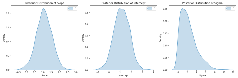 Posterior distribution plot
Method: 2 Bayesian Linear Regression using PyMC3
In this implementation, we utilize Bayesian Linear Regression with Markov Chain Monte Carlo (MCMC) sampling using PyMC3, allowing for a probabilistic interpretation of regression parameters and their uncertainties.
1. Import Necessary Libraries
Here, we import the required libraries for the task. These libraries include os, pytensor, pymc, numpy, and matplotlib.
C++ import os import pytensor import pymc as pm import numpy as np import matplotlib.pyplot as plt
2. Clear PyTensor Cache
PyMC uses PyTensor (formerly Theano) as the backend for running computations. We clear the cache to avoid any potential issues with stale compiled code
C++ cache_dir = pytensor.config.compiledir os.system(f'rm -rf {cache_dir}') 3. Set Random Seed and Generate Synthetic Data
We combine setting the random seed and generating synthetic data in this step. The random seed ensures reproducibility, and the synthetic data is generated for the linear regression model.
C++ np.random.seed(0) X = np.linspace(0, 10, 100) # Independent variable true_slope = 2 true_intercept = 1 Y = true_intercept + true_slope * X + np.random.normal(0, 1, size=100) # Dependent variable
4. Define the Bayesian Model
Now, we define the Bayesian model using PyMC. Here, we specify the priors for the model parameters (slope, intercept, and sigma), and the likelihood function for the observed data.
C++ with pm.Model() as model: slope = pm.Normal('slope', mu=0, sigma=10) intercept = pm.Normal('intercept', mu=0, sigma=10) sigma = pm.HalfNormal('sigma', sigma=1) # Prior for standard deviation of the noise # Expected value of outcome (linear model) mu = intercept + slope * X # Likelihood (observed data) Y_obs = pm.Normal('Y_obs', mu=mu, sigma=sigma, observed=Y) 5. Sample from the Posterior
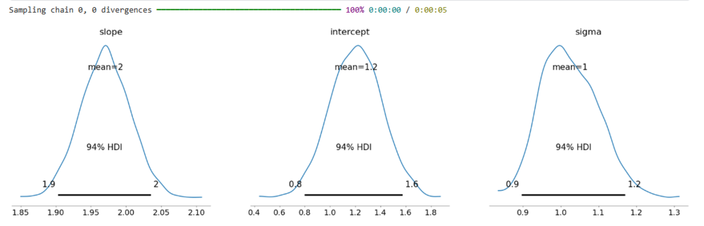
After defining the model, we sample from the posterior using MCMC (Markov Chain Monte Carlo). The pm.sample() function draws samples from the posterior distributions of the model parameters.
- We set
draws=2000 for the number of samples, tune=1000 for tuning steps, and cores=1 to use a single core for the sampling process.
C++ trace = pm.sample(draws=2000, tune=1000, cores=1, chains=1, return_inferencedata=True)
6. Plot the Posterior Distributions
Finally, we plot the posterior distributions of the parameters (slope, intercept, and sigma) to visualize the uncertainty in their estimates. pm.plot_posterior()plots the distributions, showing the most likely values for each parameter.
C++ pm.plot_posterior(trace, var_names=['slope', 'intercept', 'sigma']) plt.show()
Output
Advantages of Bayesian Regression
- Effective for small datasets: Works well when data is limited.
- Handles uncertainty: Provides probability distributions instead of point estimates.
- Flexible modeling: Can handle complex relationships and non-linearity.
- Robust against outliers: Unlike OLS, Bayesian regression reduces the impact of extreme values.
- Facilitates model selection: Computes posterior probabilities for different models.
Limitations of Bayesian Regression
- Computationally expensive: Requires advanced sampling techniques.
- Requires specifying priors: Poorly chosen priors can affect results.
- Not always necessary: For large datasets, traditional regression often performs adequately.
Similar Reads
Machine Learning Algorithms Machine learning algorithms are essentially sets of instructions that allow computers to learn from data, make predictions, and improve their performance over time without being explicitly programmed. Machine learning algorithms are broadly categorized into three types: Supervised Learning: Algorith
8 min read
Top 15 Machine Learning Algorithms Every Data Scientist Should Know in 2025 Machine Learning (ML) Algorithms are the backbone of everything from Netflix recommendations to fraud detection in financial institutions. These algorithms form the core of intelligent systems, empowering organizations to analyze patterns, predict outcomes, and automate decision-making processes. Wi
14 min read
Linear Model Regression
Ordinary Least Squares (OLS) using statsmodelsOrdinary Least Squares (OLS) is a widely used statistical method for estimating the parameters of a linear regression model. It minimizes the sum of squared residuals between observed and predicted values. In this article we will learn how to implement Ordinary Least Squares (OLS) regression using P
3 min read
Linear Regression (Python Implementation)Linear regression is a statistical method that is used to predict a continuous dependent variable i.e target variable based on one or more independent variables. This technique assumes a linear relationship between the dependent and independent variables which means the dependent variable changes pr
14 min read
Multiple Linear Regression using Python - MLLinear regression is a statistical method used for predictive analysis. It models the relationship between a dependent variable and a single independent variable by fitting a linear equation to the data. Multiple Linear Regression extends this concept by modelling the relationship between a dependen
4 min read
Polynomial Regression ( From Scratch using Python )Prerequisites Linear RegressionGradient DescentIntroductionLinear Regression finds the correlation between the dependent variable ( or target variable ) and independent variables ( or features ). In short, it is a linear model to fit the data linearly. But it fails to fit and catch the pattern in no
5 min read
Bayesian Linear RegressionLinear regression is based on the assumption that the underlying data is normally distributed and that all relevant predictor variables have a linear relationship with the outcome. But In the real world, this is not always possible, it will follows these assumptions, Bayesian regression could be the
10 min read
How to Perform Quantile Regression in PythonIn this article, we are going to see how to perform quantile regression in Python. Linear regression is defined as the statistical method that constructs a relationship between a dependent variable and an independent variable as per the given set of variables. While performing linear regression we a
4 min read
Isotonic Regression in Scikit LearnIsotonic regression is a regression technique in which the predictor variable is monotonically related to the target variable. This means that as the value of the predictor variable increases, the value of the target variable either increases or decreases in a consistent, non-oscillating manner. Mat
6 min read
Stepwise Regression in PythonStepwise regression is a method of fitting a regression model by iteratively adding or removing variables. It is used to build a model that is accurate and parsimonious, meaning that it has the smallest number of variables that can explain the data. There are two main types of stepwise regression: F
6 min read
Least Angle Regression (LARS)Regression is a supervised machine learning task that can predict continuous values (real numbers), as compared to classification, that can predict categorical or discrete values. Before we begin, if you are a beginner, I highly recommend this article. Least Angle Regression (LARS) is an algorithm u
3 min read
Linear Model Classification
Regularization
K-Nearest Neighbors (KNN)
Support Vector Machines
ML - Stochastic Gradient Descent (SGD) Stochastic Gradient Descent (SGD) is an optimization algorithm in machine learning, particularly when dealing with large datasets. It is a variant of the traditional gradient descent algorithm but offers several advantages in terms of efficiency and scalability, making it the go-to method for many d
8 min read
Decision Tree
Ensemble Learning