How to Prevent Grouped Dates In Excel Pivot Table?

Last Updated : 31 Jan, 2023

We may group dates, numbers, and text fields in a pivot table. Organize dates, for instance, by year and month. In a pivot table field, text elements can be manually selected. The selected things can then be grouped. This enables you to rapidly view the subtotals in your pivot table for a certain group of items. The built-in choices for grouping dates in a pivot table are Seconds, Minutes, Hours, Days, Months, Quarters, and Years. To establish the kind of date grouping you require, choose one or more of those possibilities. This article shows how the dates may be grouped by month and year.

Steps to Create a PivotTable

Step 1: Create an excel table with fields Date, Category, and Revenue.

Step 2: Select the data. Navigate to the Insert tab on the top of the ribbon than in the Tables group select PivotTable.

Step 3: PivotTable from the table or range dialog box appear. Here select the table range and select the new worksheet and then click on OK.

Step 4: Now you can see the Pivot table and Pivot table field pane in created. From the PivotTable fields pane, selects the Date and Revenue field.

Step 5: Now as you can see, Pivot Table is created with the Date and the revenue field.

Group Dates by Month

Step 1: Here select any date and then right-click on it. Here select the Group option.

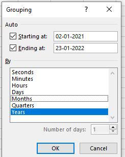
Step 2: Then Grouping dialog box will appear. Here, first fix the starting at and ending at then in the By pane select the Months option and then click on OK.

Step 3: Now you can see the table is showing only months with the revenue.

Group Dates by Years

Step 1: Now, right-click on the month and then choose a group option. Then Grouping dialog box will appear. Here first fix the starting at and ending at then in the By Pane select the Years option and then click on OK.

Step 2: Now you can see the table showing only years with the total revenue.

Group Dates by Quarters

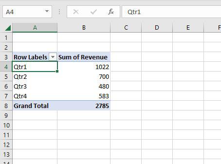
Step 1: Now, right-click on the Years and then choose a group option. Then Grouping dialog box will appear. Here first fix the starting at and ending at then in By Pane select the Quarters option and then click on OK.

Step 2: Now you can see the table showing only Quarters with the total revenue.

Group Dates by Days

Step 1: Now again right click on the Quarters and then choose a group option. Then Grouping dialog box will appear. Here first fix the starting at and ending at then in the By pane select the Days option and select Number of days. Here we are selecting 20 and then clicking on OK.

Step 2: Now you can see the table showing Dates in 20 days grouping with the revenue.

Group Dates by Seconds, Minutes, and Hours

Step 1: Now again right click on the Days and then choose a group option. Then Grouping dialog box will appear. Here first fix the starting at and ending at then in the By pane select the Seconds, Minutes, and hours options. Then click on OK.

Step 2: Now you can see the table shows 00 in seconds, minutes, and hours. Because the time is not there in the pivot table. But it shows the total revenue.