Skip to content
geeksforgeeks
  • Tutorials
    • Python
    • Java
    • Data Structures & Algorithms
    • ML & Data Science
    • Interview Corner
    • Programming Languages
    • Web Development
    • CS Subjects
    • DevOps And Linux
    • School Learning
    • Practice Coding Problems
  • Courses
    • DSA to Development
    • Get IBM Certification
    • Newly Launched!
      • Master Django Framework
      • Become AWS Certified
    • For Working Professionals
      • Interview 101: DSA & System Design
      • Data Science Training Program
      • JAVA Backend Development (Live)
      • DevOps Engineering (LIVE)
      • Data Structures & Algorithms in Python
    • For Students
      • Placement Preparation Course
      • Data Science (Live)
      • Data Structure & Algorithm-Self Paced (C++/JAVA)
      • Master Competitive Programming (Live)
      • Full Stack Development with React & Node JS (Live)
    • Full Stack Development
    • Data Science Program
    • All Courses
  • Data Visualization
  • Statistics in R
  • Machine Learning in R
  • Data Science in R
  • Packages in R
  • Data Types
  • String
  • Array
  • Vector
  • Lists
  • Matrices
  • Oops in R
Open In App
Next Article:
Beta Distribution in R
Next article icon

Beta Distribution in R

Last Updated : 15 Feb, 2022
Comments
Improve
Suggest changes
Like Article
Like
Report

A distribution in statistics is a function that shows the possible values for a variable and how often they occur in the particular experiment or dataset. Beta distribution is one type of probability distribution that represents all the possible outcomes of the dataset. Beta distribution basically shows the probability of probabilities, where α and β, can take any values which depend on the probability of success/failure.

The general formula for the probability density function of the beta distribution is:

f(x)=\frac{(x-a)^{p-1}(b-x)^{q-1}}{B(p,q)(b-a)^{p+q-1})}\hspace{.3in} a \le x \le b; p, q > 0.   

where ,

  • p and q are the shape parameters
  • a and b are lower and upper bound
  • a≤x≤b
  • p,q>0
  • B(p,q) is the beta function

To understand the beta distribution in R specifically, we will learn about beta functions. Beta function is a component of beta distribution (the beta function in R can be implemented using the beta (a,b) function) which include these dbeta , pbeta , qbeta , and rbeta which are the functions of the Beta distribution.

Beta function defines as :

B(\alpha ,\beta )=\int_{0}^{1} t^{^{\alpha -1}}(1-t)^{\beta } dt

The case where a = 0 and b = 1 is called the standard beta distribution. Hence standard beta distribution is :

f(x)=\frac{(x)^{p-1}(1-x)^{q-1}}{B(p,q)}  \displaystyle \propto {(x)^{p-1}}{(1-x)^{q-1}}\hspace{.3in} 0 \le x \le 1; p, q > 0.   

Through beta distribution, we can also find out the measures of central tendency like mean, median mode, and also measures of statistical dispersion like variance.

Why Beta Distribution?

Why we might actually want to choose the beta distribution to specify prior knowledge about theta, one of the major reasons is that this distribution is defined in the range of  [0,1] so a beta distribution is a very natural distribution to use when we are talking about probabilities and we want to specify about a prior knowledge of the probabilities of something accruing.

Range of beliefs in Beta Distribution 

The range of beliefs is that we can actually define a great set of quite a large range by changing the parameters of p and q i.e. shape parameters.

Let us take an example to understand it better.

S.no.pq

1

0.50.5

2

0.51

3

11

4

33

Let us start when both p and q are 0.5. We put 1/2 in this equation :

f(x)={(x)^{p-1}}{(1-x)^{q-1}}\hspace{.3in} 0 \le x \le 1; p, q > 0.   

After this it becomes f(x | p,q)  = {(x)^{-1/2}(1-x)^{-1/2}}\hspace{.3in} 0 \le x \le 1; p, q > 0.             

then we can also write this equation like :

 f(x |p,q) = \frac {1}{(x)^{1/2}(1-x)^{1/2}}\hspace{.3in} 0 \le x \le 1; p, q > 0.   

Hence, from the above equation we observed that if x becomes zero or 1 , then we have infinity. Then we will calculate the points for all p and q values. The PDF (Probability distribution function) of Beta distribution can be formed in three shapes from the above observations U-shaped with asymptotic ends, bell-shaped, strictly increasing/decreasing or even straight lines. As you change value of p or q, the shape of the distribution changes. 

Hence, the graph will look like this :

Now, let's plot the Beta distribution functions in R in order to understand them better. Firstly, plot Beta Density and after that all other functions.

Beta density

For plotting the beta density as we know that it will lie between the range of (0,1). We are using one dbeta and plot function in the plot.

 Syntax: dbeta(xvalues,alpha,beta)

Example 1: Here, we can observe that Plot for Beta Density(1,1)  where we can observe the uniform distribution between 0 and 1.

R
# Creating the Sequence gfg = seq(0, 1, by = 0.1)  # Plotting the beta density plot(gfg, dbeta(gfg, 1,1), xlab="X",      ylab = "Beta Density", type = "l",      col = "Red") 


Output:


Plot for Beta Density(1,1)


Example 2: Here, we can observe that Plot for Beta Density(2,1) where we can observe linearly increasing function, In the above plot we can see that is the points are more likely to be near 1 than 0 and they go up in a proportional manner. If we just change the plot from (2,1) to (1,2) we can see that is the points are more likely to be near 0 than 1.


R
# Creating the Sequence gfg = seq(0,1, by=0.1)  # Case 2 plot(gfg, dbeta(gfg, 2,1), xlab="X",      ylab = "Beta Density", type = "l",      col = "Red")  

Output:

Plot for Beta Density(2,1)  

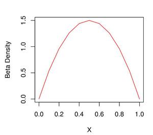
Example 3: Here, we can observe that Plot for Beta Density(2,2) where we can observe the quadratic function values between nearly 0 and 1 but most likely to have a value near 1/2.

R
# Creating the Sequence gfg = seq(0,1, by=0.1)  # Case 3 plot(gfg, dbeta(gfg, 2,2), xlab = "X",      ylab = "Beta Density", type = "l",      col = "Red")  

Output:

Plot for Beta Density(2,2) 

Cumulative Distributive Functions

You can refer to this link about the functions of Beta Distribution Functions.

Here in our case, the data that we have shows the average which can take any numerical values between 0 and 1 as you can see 0,1 are parameters in sequence in line no.3 in the above code, so through beta distribution, we depict a bounded continuous distribution with values between 0 and 1, and primarily model the uncertainty about the probability of success of a random experiment, which in our case, is the probability of probabilities having a particular average.

Because of this, it is often used in uncertainty problems associated with proportions, frequency or percentages.

R
# The Beta Distribution plr.data <- data.frame(   player_avg <- c(seq(0, 1, by = 0.025)),   stringsAsFactors = FALSE )  # Print the data frame.             print(plr.data) print(plr.data$player_avg) by1 <- dbeta(plr.data$player_avg, shape1 = 5, shape2 = 8) par(mar = rep(2,4)) plot(by1)  # Cummilative distribution function  by2<- pbeta(plr.data$player_avg, shape1 = 4, shape2 = 6)  par(mar = rep(2,4)) plot(by2)  # Inverse Cummilative distribution function  by3 <- qbeta(plr.data$player_avg, shape1 = 4, shape2 = 6) par(mar = rep(2,4)) plot(by3)  b4 <- rbeta(plr.data$player_avg, shape1 = 5, shape2 = 8) par(mar = rep(2,4)) plot(density(b4), main = "Rbeta Plot") 


Output:


Next Article
Beta Distribution in R

Y

yashisrivastav
Improve
Article Tags :
  • R Language
  • R-Statistics

Similar Reads

    Real-life Applications of Beta Distribution
    Beta distribution is a continuous probability distribution that is lined up with the range [0, 1]. It is widely used in applying Bayesian statistics and reliability analysis for showing percentages and rates. The article introduces the Beta distribution in simple words and goes across different appl
    6 min read
    Curve Fitting in R
    In this article, we will discuss how to fit a curve to a dataframe in the R Programming language. Curve fitting is one of the basic functions of statistical analysis. It helps us in determining the trends and data and helps us in the prediction of unknown data based on a regression model/function.
    4 min read
    Built-in Constants in R
    R is a popular programming language and environment for statistical computing and graphics, providing a variety of built-in constants that are useful for different types of data analysis and scientific computations. Understanding these constants is essential for efficient coding and accurate results
    3 min read
    as.numeric() Function in R
    The as.numeric() function in R is a crucial tool for data manipulation, allowing users to convert data into numeric form, which is essential for performing mathematical operations and statistical analysis. Overview of the as.numeric() FunctionThe as. numeric() function is part of R's base package an
    3 min read
    Introduction to R Studio
    R Studio is an integrated development environment(IDE) for R. IDE is a GUI, where you can write your quotes, see the results and also see the variables that are generated during the course of programming.  R Studio is available as both Open source and Commercial software.R Studio is also available a
    4 min read
geeksforgeeks-footer-logo
Corporate & Communications Address:
A-143, 7th Floor, Sovereign Corporate Tower, Sector- 136, Noida, Uttar Pradesh (201305)
Registered Address:
K 061, Tower K, Gulshan Vivante Apartment, Sector 137, Noida, Gautam Buddh Nagar, Uttar Pradesh, 201305
GFG App on Play Store GFG App on App Store
Advertise with us
  • Company
  • About Us
  • Legal
  • Privacy Policy
  • In Media
  • Contact Us
  • Advertise with us
  • GFG Corporate Solution
  • Placement Training Program
  • Languages
  • Python
  • Java
  • C++
  • PHP
  • GoLang
  • SQL
  • R Language
  • Android Tutorial
  • Tutorials Archive
  • DSA
  • Data Structures
  • Algorithms
  • DSA for Beginners
  • Basic DSA Problems
  • DSA Roadmap
  • Top 100 DSA Interview Problems
  • DSA Roadmap by Sandeep Jain
  • All Cheat Sheets
  • Data Science & ML
  • Data Science With Python
  • Data Science For Beginner
  • Machine Learning
  • ML Maths
  • Data Visualisation
  • Pandas
  • NumPy
  • NLP
  • Deep Learning
  • Web Technologies
  • HTML
  • CSS
  • JavaScript
  • TypeScript
  • ReactJS
  • NextJS
  • Bootstrap
  • Web Design
  • Python Tutorial
  • Python Programming Examples
  • Python Projects
  • Python Tkinter
  • Python Web Scraping
  • OpenCV Tutorial
  • Python Interview Question
  • Django
  • Computer Science
  • Operating Systems
  • Computer Network
  • Database Management System
  • Software Engineering
  • Digital Logic Design
  • Engineering Maths
  • Software Development
  • Software Testing
  • DevOps
  • Git
  • Linux
  • AWS
  • Docker
  • Kubernetes
  • Azure
  • GCP
  • DevOps Roadmap
  • System Design
  • High Level Design
  • Low Level Design
  • UML Diagrams
  • Interview Guide
  • Design Patterns
  • OOAD
  • System Design Bootcamp
  • Interview Questions
  • Inteview Preparation
  • Competitive Programming
  • Top DS or Algo for CP
  • Company-Wise Recruitment Process
  • Company-Wise Preparation
  • Aptitude Preparation
  • Puzzles
  • School Subjects
  • Mathematics
  • Physics
  • Chemistry
  • Biology
  • Social Science
  • English Grammar
  • Commerce
  • World GK
  • GeeksforGeeks Videos
  • DSA
  • Python
  • Java
  • C++
  • Web Development
  • Data Science
  • CS Subjects
@GeeksforGeeks, Sanchhaya Education Private Limited, All rights reserved
We use cookies to ensure you have the best browsing experience on our website. By using our site, you acknowledge that you have read and understood our Cookie Policy & Privacy Policy
Lightbox
Improvement
Suggest Changes
Help us improve. Share your suggestions to enhance the article. Contribute your expertise and make a difference in the GeeksforGeeks portal.
geeksforgeeks-suggest-icon
Create Improvement
Enhance the article with your expertise. Contribute to the GeeksforGeeks community and help create better learning resources for all.
geeksforgeeks-improvement-icon
Suggest Changes
min 4 words, max Words Limit:1000

Thank You!

Your suggestions are valuable to us.

What kind of Experience do you want to share?

Interview Experiences
Admission Experiences
Career Journeys
Work Experiences
Campus Experiences
Competitive Exam Experiences