Back Propagation with TensorFlow

Last Updated : 26 May, 2025

Backpropagation is an algorithm that helps neural networks learn by reducing the error between the predicted and actual outputs. It adjusts the model's weights and biases based on the calculated error. It works in two steps:

Feedforward Pass: The input data moves from the input layer to the output layer passing through hidden layers. Each layer performs calculations and applies activation functions.
Backward Pass: The model calculates how much each weight contributes to the error and updates the weights to minimize the loss. This process continues until the model produces a accurate prediction

TensorFlow is one of the most popular deep learning libraries which helps in efficient training of deep neural network and in this article we will focus on the implementation of backpropagation in tensorflow.

To install TensorFlow use this command:

pip install tensorflow

1. Importing Libraries

Here we are importing all the important libraries need to build the model. The following libraries are Numpy, Sklearn and TensorFlow.

Python

import tensorflow as tf import numpy as np from sklearn import datasets from sklearn.model_selection import train_test_split

2. Loading the dataset

We'll use the Iris dataset a popular dataset in machine learning that contains 150 samples and 4 features (sepal length, sepal width, petal length, petal width)

Python

iris = datasets.load_iris() X = iris.data y = iris.target

3. Training and Testing the model

Now we divide the the iris dataset into training set (80%) and testing set(20%) to facilitate the development and evaluation of the model. The random_state argument is set for reproducibility, ensuring that same split is obtained each time the code is run.

Python

X_train, X_test, y_train, y_test = train_test_split( X, y, test_size=0.2, random_state=42)

4. Defining a machine learning model

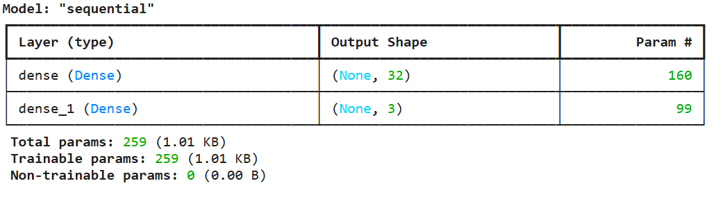
In this step we are defining a model using tensorflow's Keras. The model consist of two layers:

Dense Layer: A hidden layer with the ReLU activation function and an input shape that matches the number of the features in the training data.
Output Layer: An output layer has three neurons and uses a softmax activation function to produce class probabilities.

Python

hidden_layer_size = 32 model = tf.keras.Sequential([     tf.keras.layers.Dense(hidden_layer_size, activation='relu', input_shape=(X_train.shape[1],)),     tf.keras.layers.Dense(3, activation='softmax')  # 3 classes for Iris dataset ])  model.summary()

Output:

5. Loss function and optimizer

The model needs a loss function to measure how far the predictions are from the actual labels and an optimizer to update the weights.

Sparse Categorical Crossentropy: It is a loss function used in classification tasks where target and labels are integers. It calculates the cross-entropy loss between the predicted class probabilities and true class labels, automatically converting integer labels to one-hot encoded vectors internally.
Stochastic Gradient Descent(SGD): It is an optimization algorithm used for training models. It updates model parameters using small, randomly sampled subsets of the training data, which introduces randomness and helps the model converge to a solution faster and potentially escape local minima.

Python

learning_rate = 0.01 epochs = 1000  loss_fn = tf.keras.losses.SparseCategoricalCrossentropy() optimizer = tf.keras.optimizers.SGD(learning_rate)

6. Implementing Backpropagation

Now let's train the model using backpropagation. The GradientTape context records the forward pass and automatically calculates gradients during the backward pass.

GradientTape() context automatically tracks all mathematical operations applied to tensors.
Labels are converted into tensors with dtype=tf.int32 to ensure compatibility with the loss function.
logits are the raw predictions from the model before applying the softmax activation.
loss_value is calculated using the loss function.
tape.gradient() method calculates the gradients of the loss with respect to the model parameters.
apply_gradients() method updates the weights using the optimizer.
The model prints the loss value every 100 epochs to track the training process.

Python

y_train = tf.convert_to_tensor(y_train, dtype=tf.int32)  for epoch in range(epochs):     with tf.GradientTape() as tape:         logits = model(X_train)           loss_value = loss_fn(y_train, logits)       grads = tape.gradient(loss_value, model.trainable_variables)      optimizer.apply_gradients(zip(grads, model.trainable_variables))      if (epoch + 1) % 100 == 0:         print(f"Epoch {epoch + 1}/{epochs}, Loss: {loss_value.numpy()}")

Output:

We can see that our model is trained with minimal loss hence we can use it.

Back Propagation with TensorFlow

anvi27

Improve

Article Tags :

Practice Tags :

Machine Learning

Back Propagation with TensorFlow

1. Importing Libraries

2. Loading the dataset

3. Training and Testing the model

4. Defining a machine learning model

5. Loss function and optimizer

6. Implementing Backpropagation

Similar Reads